random_rewire

graph_tool.generation.random_rewire(g, model='configuration', n_iter=10, edge_sweep=True, parallel_edges=False, self_loops=False, configuration=True, edge_probs=None, block_membership=None, cache_probs=True, persist=False, pin=None, ret_fail=False, verbose=False)

Shuffle the graph in-place, following a variety of possible statistical models, chosen via the parameter model.

Parameters:

gGraph

Graph to be shuffled. The graph will be modified.

modelstring (optional, default: "configuration")

The following statistical models can be chosen, which determine how the edges are rewired.

erdos

The edges will be rewired entirely randomly, and the resulting graph will correspond to the \(G(N,E)\) Erdős–Rényi model.

configuration

The edges will be rewired randomly, but the degree sequence of the graph will remain unmodified.

constrained-configuration

The edges will be rewired randomly, but both the degree sequence of the graph and the vertex-vertex (in,out)-degree correlations will remain exactly preserved. If the block_membership parameter is passed, the block variables at the endpoints of the edges will be preserved, instead of the degree-degree correlation.

probabilistic-configuration

This is similar to constrained-configuration, but the vertex-vertex correlations are not preserved, but are instead sampled from an arbitrary degree-based probabilistic model specified via the edge_probs parameter. The degree-sequence is preserved.

blockmodel-degree

This is just like probabilistic-configuration, but the values passed to the edge_probs function will correspond to the block membership values specified by the block_membership parameter.

blockmodel

This is just like blockmodel-degree, but the degree sequence is not preserved during rewiring.

blockmodel-micro

This is like blockmodel, but the exact number of edges between groups is preserved as well.

n_iterint (optional, default: 10)

Number of iterations. If edge_sweep == True, each iteration corresponds to an entire “sweep” over all edges. Otherwise this corresponds to the total number of edges which are randomly chosen for a swap attempt (which may repeat).

edge_sweepbool (optional, default: True)

If True, each iteration will perform an entire “sweep” over the edges, where each edge is visited once in random order, and a edge swap is attempted.

parallel_edgesbool (optional, default: False)

If True, parallel edges are allowed.

self_loopsbool (optional, default: False)

If True, self-loops are allowed.

configurationbool (optional, default: True)

If True, graphs are sampled from the corresponding maximum-entropy ensemble of configurations (i.e. distinguishable half-edge pairings), otherwise they are sampled from the maximum-entropy ensemble of graphs (i.e. indistinguishable half-edge pairings). The distinction is only relevant if parallel edges are allowed.

edge_probsfunction or sequence of triples (optional, default: None)

A function which determines the edge probabilities in the graph. In general it should have the following signature:

def prob(r, s):
    ...
    return p

where the return value should be a non-negative scalar.

Alternatively, this parameter can be a list of triples of the form (r, s, p), with the same meaning as the r, s and p values above. If a given (r, s) combination is not present in this list, the corresponding value of p is assumed to be zero. If the same (r, s) combination appears more than once, their p values will be summed together. This is useful when the correlation matrix is sparse, i.e. most entries are zero.

If model == probabilistic-configuration the parameters r and s correspond respectively to the (in, out)-degree pair of the source vertex of an edge, and the (in,out)-degree pair of the target of the same edge (for undirected graphs, both parameters are scalars instead). The value of p should be a number proportional to the probability of such an edge existing in the generated graph.

If model == blockmodel-degree or model == blockmodel, the r and s values passed to the function will be the block values of the respective vertices, as specified via the block_membership parameter. The value of p should be a number proportional to the probability of such an edge existing in the generated graph.

block_membershipVertexPropertyMap (optional, default: None)

If supplied, the graph will be rewired to conform to a blockmodel ensemble. The value must be a vertex property map which defines the block of each vertex.

cache_probsbool (optional, default: True)

If True, the probabilities returned by the edge_probs parameter will be cached internally. This is crucial for good performance, since in this case the supplied python function is called only a few times, and not at every attempted edge rewire move. However, in the case were the different parameter combinations to the probability function is very large, the memory and time requirements to keep the cache may not be worthwhile.

persistbool (optional, default: False)

If True, an edge swap which is rejected will be attempted again until it succeeds. This may improve the quality of the shuffling for some probabilistic models, and should be sufficiently fast for sparse graphs, but otherwise it may result in many repeated attempts for certain corner-cases in which edges are difficult to swap.

pinEdgePropertyMap (optional, default: None)

Edge property map which, if provided, specifies which edges are allowed to be rewired. Edges for which the property value is 1 (or True) will be left unmodified in the graph.

verbosebool (optional, default: False)

If True, verbose information is displayed.

Returns:

rejection_countint

Number of rejected edge moves (due to parallel edges or self-loops, or the probabilistic model used).

See also

random_graph

random graph generation

Notes

This algorithm iterates through all the edges in the network and tries to swap its target or source with the target or source of another edge. The selected canditate swaps are chosen according to the model parameter.

Note

If parallel_edges = False, parallel edges are not placed during rewiring. In this case, the returned graph will be a uncorrelated sample from the desired ensemble only if n_iter is sufficiently large. The algorithm implements an efficient Markov chain based on edge swaps, with a mixing time which depends on the degree distribution and correlations desired. If degree probabilistic correlations are provided, the mixing time tends to be larger.

If model is either “probabilistic-configuration”, “blockmodel” or “blockmodel-degree”, the Markov chain still needs to be mixed, even if parallel edges and self-loops are allowed. In this case the Markov chain is implemented using the Metropolis-Hastings [metropolis-equations-1953] [hastings-monte-carlo-1970] acceptance/rejection algorithm. It will eventually converge to the desired probabilities for sufficiently large values of n_iter.

Each edge is tentatively swapped once per iteration, so the overall complexity is \(O(V + E \times \text{n-iter})\). If edge_sweep == False, the complexity becomes \(O(V + E + \text{n-iter})\).

References

[metropolis-equations-1953]

Metropolis, N.; Rosenbluth, A.W.; Rosenbluth, M.N.; Teller, A.H.; Teller, E. “Equations of State Calculations by Fast Computing Machines”. Journal of Chemical Physics 21 (6): 1087-1092 (1953). DOI: 10.1063/1.1699114 [sci-hub, @tor]

[hastings-monte-carlo-1970]

Hastings, W.K. “Monte Carlo Sampling Methods Using Markov Chains and Their Applications”. Biometrika 57 (1): 97-109 (1970). DOI: 10.1093/biomet/57.1.97 [sci-hub, @tor]

[holland-stochastic-1983]

Paul W. Holland, Kathryn Blackmond Laskey, and Samuel Leinhardt, “Stochastic blockmodels: First steps,” Social Networks 5, no. 2: 109-13 (1983) DOI: 10.1016/0378-8733(83)90021-7 [sci-hub, @tor]

[karrer-stochastic-2011]

Brian Karrer and M. E. J. Newman, “Stochastic blockmodels and community structure in networks,” Physical Review E 83, no. 1: 016107 (2011) DOI: 10.1103/PhysRevE.83.016107 [sci-hub, @tor] arXiv: 1008.3926

Examples

Some small graphs for visualization.

>>> g, pos = gt.triangulation(np.random.random((1000,2)))
>>> pos = gt.arf_layout(g)
>>> gt.graph_draw(g, pos=pos, output="rewire_orig.pdf")
<...>

>>> ret = gt.random_rewire(g, "constrained-configuration")
>>> pos = gt.arf_layout(g)
>>> gt.graph_draw(g, pos=pos, output="rewire_corr.pdf")
<...>

>>> ret = gt.random_rewire(g)
>>> pos = gt.arf_layout(g)
>>> gt.graph_draw(g, pos=pos, output="rewire_uncorr.pdf")
<...>

>>> ret = gt.random_rewire(g, "erdos")
>>> pos = gt.arf_layout(g)
>>> gt.graph_draw(g, pos=pos, output="rewire_erdos.pdf")
<...>

Some ridiculograms :

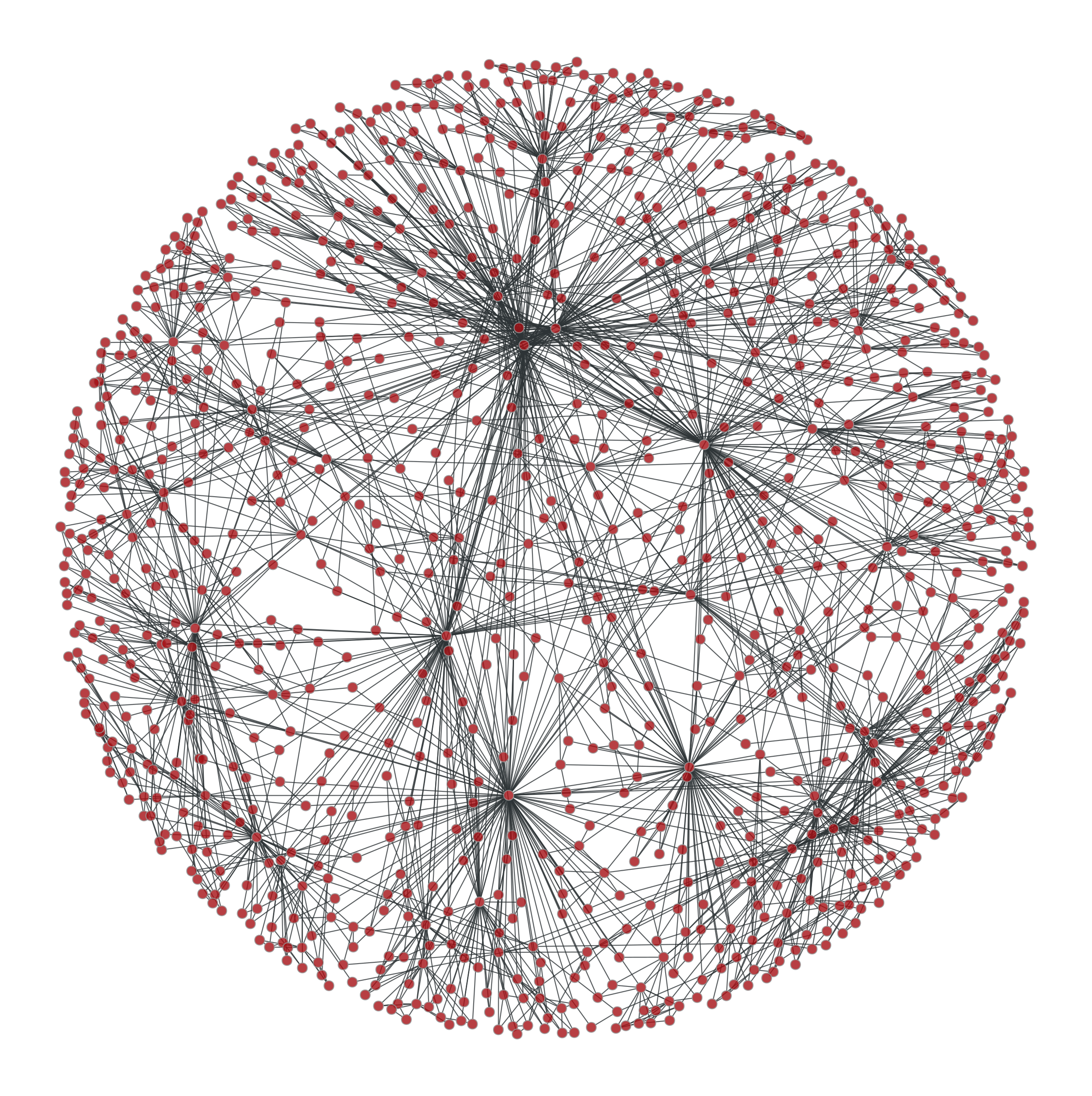
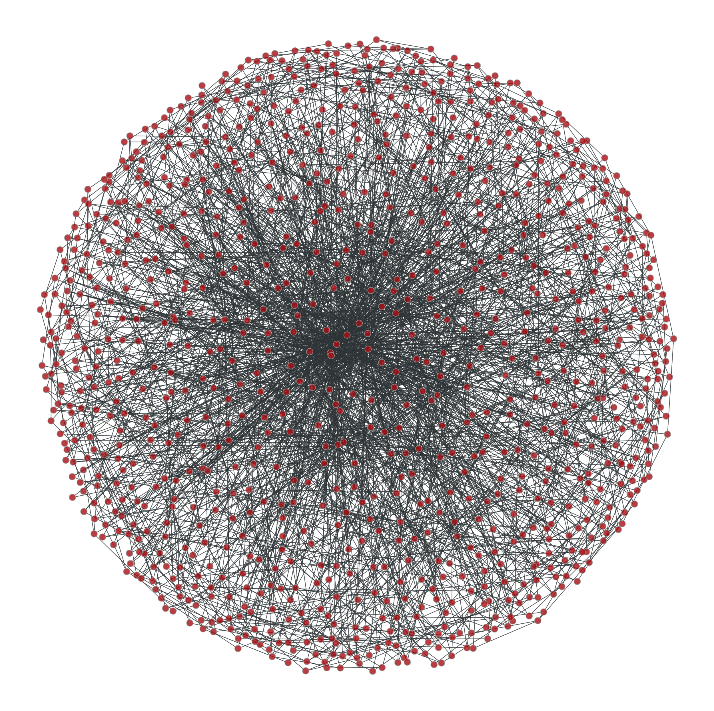
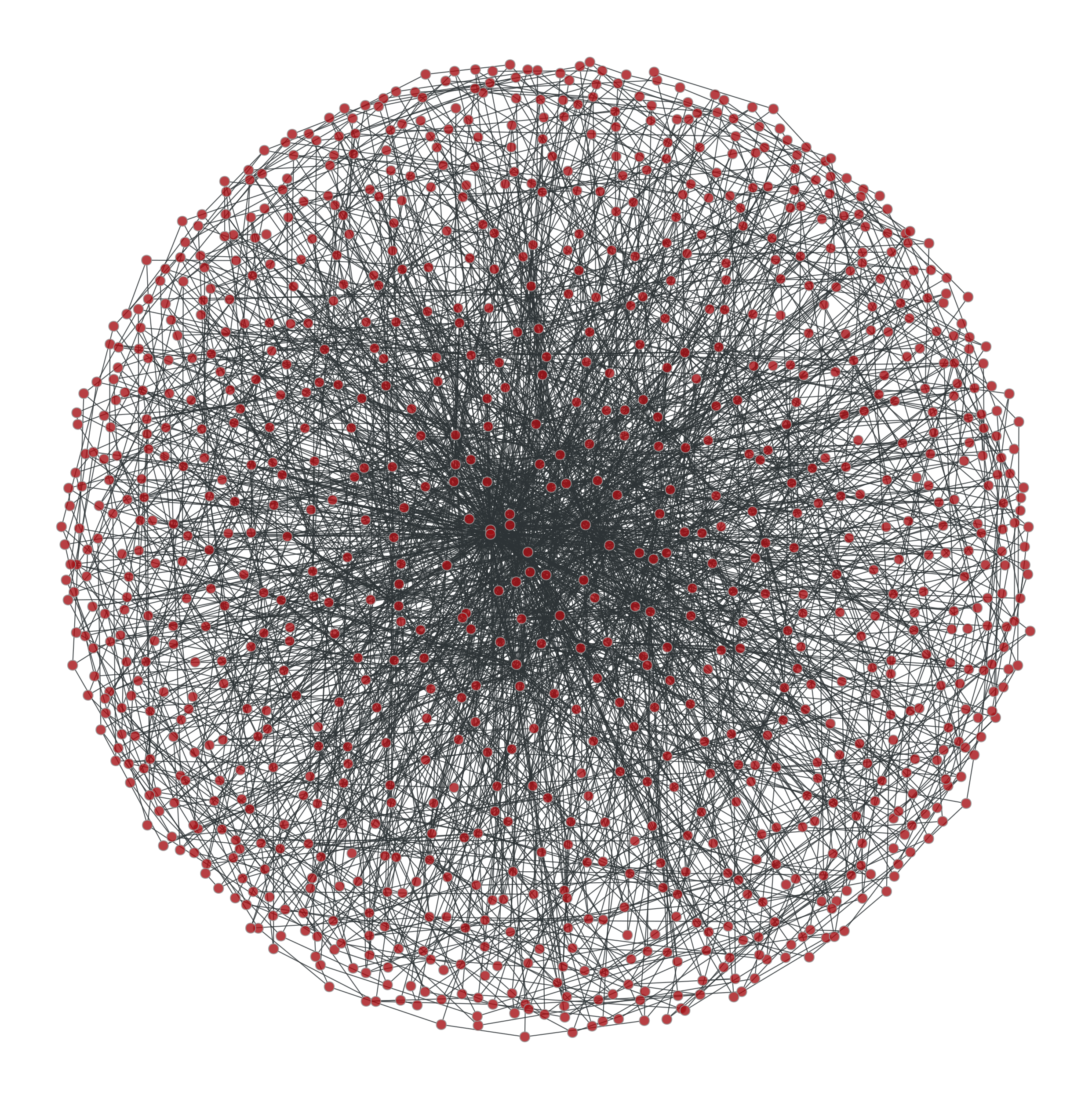
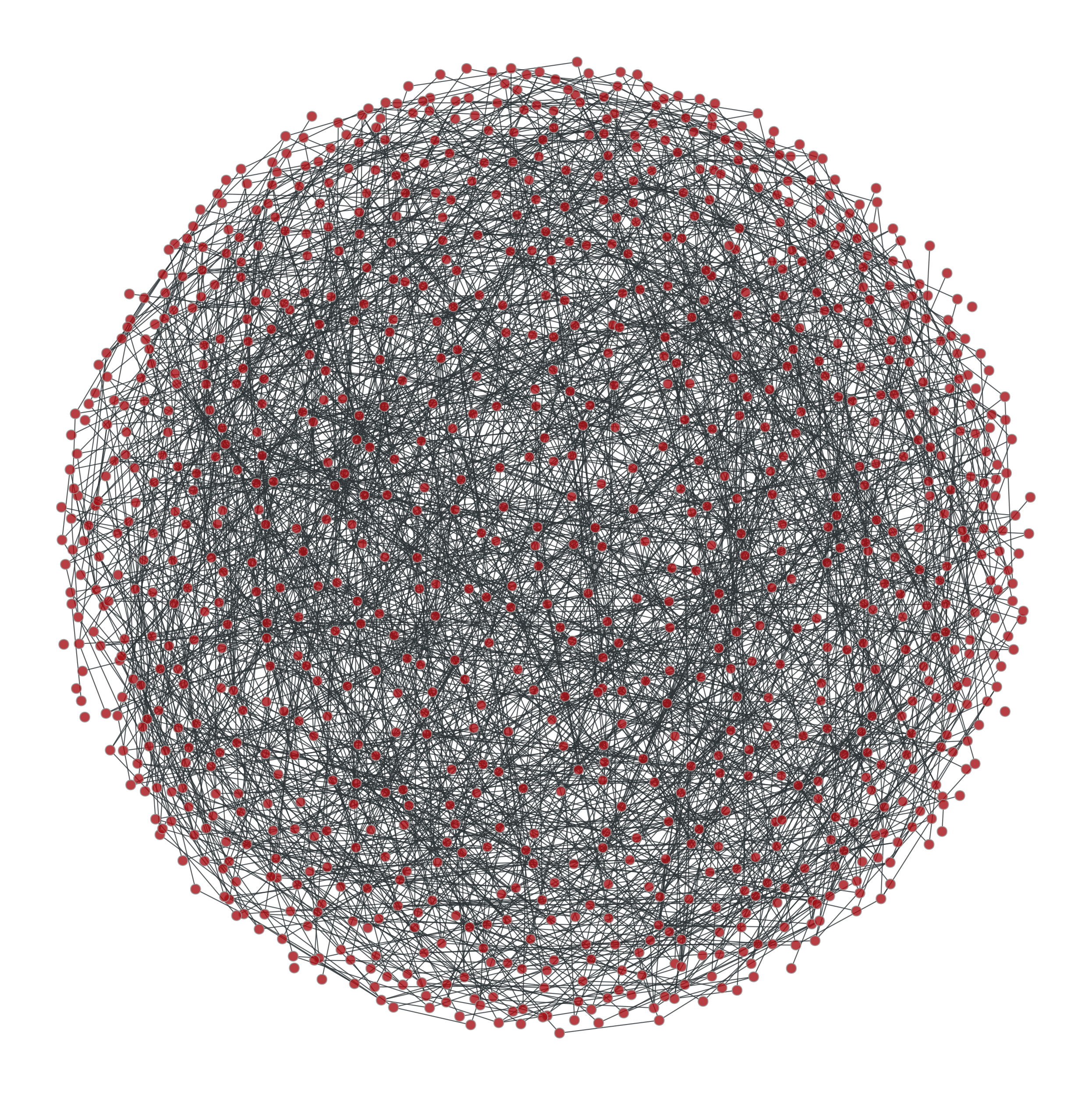
From left to right: Original graph; Shuffled graph, with degree correlations; Shuffled graph, without degree correlations; Shuffled graph, with random degrees.

We can try with larger graphs to get better statistics, as follows.

>>> def sample_k(max):
...     accept = False
...     while not accept:
...         k = np.random.randint(1,max+1)
...         accept = np.random.random() < 1.0/k
...     return k
>>> figure(figsize=(8,3))
<...>
>>> g = gt.random_graph(30000, lambda: sample_k(20), model="probabilistic-configuration",
...                     edge_probs=lambda i, j: exp(abs(i-j)), directed=False,
...                     n_iter=100)
>>> corr = gt.avg_neighbor_corr(g, "out", "out")
>>> errorbar(corr[2][:-1], corr[0], yerr=corr[1], fmt="o-", label="Original")
<...>
>>> ret = gt.random_rewire(g, "constrained-configuration")
>>> corr = gt.avg_neighbor_corr(g, "out", "out")
>>> errorbar(corr[2][:-1], corr[0], yerr=corr[1], fmt="*", label="Correlated")
<...>
>>> ret = gt.random_rewire(g)
>>> corr = gt.avg_neighbor_corr(g, "out", "out")
>>> errorbar(corr[2][:-1], corr[0], yerr=corr[1], fmt="o-", label="Uncorrelated")
<...>
>>> ret = gt.random_rewire(g, "erdos")
>>> corr = gt.avg_neighbor_corr(g, "out", "out")
>>> errorbar(corr[2][:-1], corr[0], yerr=corr[1], fmt="o-", label=r"Erd\H{o}s")
<...>
>>> xlabel("$k$")
Text(...)
>>> ylabel(r"$\left<k_{nn}\right>$")
Text(...)
>>> legend(loc='center left', bbox_to_anchor=(1, 0.5))
<...>
>>> tight_layout()
>>> box = gca().get_position()
>>> gca().set_position([box.x0, box.y0, box.width * 0.7, box.height])
>>> savefig("shuffled-stats.svg")

Average degree correlations for the different shuffled and non-shuffled graphs. The shuffled graph with correlations displays exactly the same correlation as the original graph.

Now let’s do it for a directed graph. See random_graph() for more details.

>>> def sample_k(max):
...     accept = False
...     while not accept:
...         k = np.random.randint(1,max+1)
...         accept = np.random.random() < 1.0/k
...     return k
>>> p = scipy.stats.poisson
>>> g = gt.random_graph(20000, lambda: (sample_k(19), sample_k(19)),
...                     model="probabilistic-configuration",
...                     edge_probs=lambda a, b: (p.pmf(a[0], b[1]) * p.pmf(a[1], 20 - b[0])),
...                     n_iter=100)
>>> figure(figsize=(9,3))
<...>
>>> corr = gt.avg_neighbor_corr(g, "in", "out")
>>> errorbar(corr[2][:-1], corr[0], yerr=corr[1], fmt="o-",
...          label=r"$\left<\text{o}\right>$ vs i")
<...>
>>> corr = gt.avg_neighbor_corr(g, "out", "in")
>>> errorbar(corr[2][:-1], corr[0], yerr=corr[1], fmt="o-",
...          label=r"$\left<\text{i}\right>$ vs o")
<...>
>>> ret = gt.random_rewire(g, "constrained-configuration")
>>> corr = gt.avg_neighbor_corr(g, "in", "out")
>>> errorbar(corr[2][:-1], corr[0], yerr=corr[1], fmt="o-",
...          label=r"$\left<\text{o}\right>$ vs i, corr.")
<...>
>>> corr = gt.avg_neighbor_corr(g, "out", "in")
>>> errorbar(corr[2][:-1], corr[0], yerr=corr[1], fmt="o-",
...          label=r"$\left<\text{i}\right>$ vs o, corr.")
<...>
>>> ret = gt.random_rewire(g, "configuration")
>>> corr = gt.avg_neighbor_corr(g, "in", "out")
>>> errorbar(corr[2][:-1], corr[0], yerr=corr[1], fmt="o-",
...          label=r"$\left<\text{o}\right>$ vs i, uncorr.")
<...>
>>> corr = gt.avg_neighbor_corr(g, "out", "in")
>>> errorbar(corr[2][:-1], corr[0], yerr=corr[1], fmt="o-",
...          label=r"$\left<\text{i}\right>$ vs o, uncorr.")
<...>
>>> legend(loc='center left', bbox_to_anchor=(1, 0.5))
<...>
>>> xlabel("Source degree")
Text(...)
>>> ylabel("Average target degree")
Text(...)
>>> tight_layout()
>>> box = gca().get_position()
>>> gca().set_position([box.x0, box.y0, box.width * 0.55, box.height])
>>> savefig("shuffled-deg-corr-dir.svg")

Average degree correlations for the different shuffled and non-shuffled directed graphs. The shuffled graph with correlations displays exactly the same correlation as the original graph.