min_st_cut#
- graph_tool.flow.min_st_cut(g, source, capacity, residual)[source]#
Get the minimum source-target cut, given the residual capacity of the edges.
- Parameters:
- g
Graph Graph to be used.
- sourceVertex
The source vertex.
- capacity
EdgePropertyMap Edge property map with the edge capacities.
- residual
EdgePropertyMap Edge property map with the residual capacities (capacity - flow).
- g
- Returns:
- partition
EdgePropertyMap Boolean-valued vertex property map with the cut partition. Vertices with value True belong to the source side of the cut.
- partition
Notes
The source-side of the cut set is obtained by following all vertices which are reachable from the source in the residual graph (i.e. via edges with nonzero residual capacity, and reversed edges with nonzero flow).
This algorithm runs in \(O(V+E)\) time.
References
[max-flow-min-cut]Examples
>>> g = gt.load_graph("../mincut-st-example.xml.gz")
>>> cap = g.edge_properties["weight"]
>>> src, tgt = g.vertex(0), g.vertex(7)
>>> res = gt.boykov_kolmogorov_max_flow(g, src, tgt, cap)
>>> part = gt.min_st_cut(g, src, cap, res)
>>> mc = sum([cap[e] - res[e] for e in g.edges() if part[e.source()] != part[e.target()]])
>>> print(mc)
3
>>> pos = g.vertex_properties["pos"]
>>> res.a = cap.a - res.a  # the actual flow
>>> gt.graph_draw(g, pos=pos, edge_pen_width=gt.prop_to_size(cap, mi=3, ma=10, power=1),
...               edge_text=res, vertex_fill_color=part, vertex_text=g.vertex_index,
...               vertex_font_size=18, edge_font_size=18, output="example-min-st-cut.pdf")
<...>
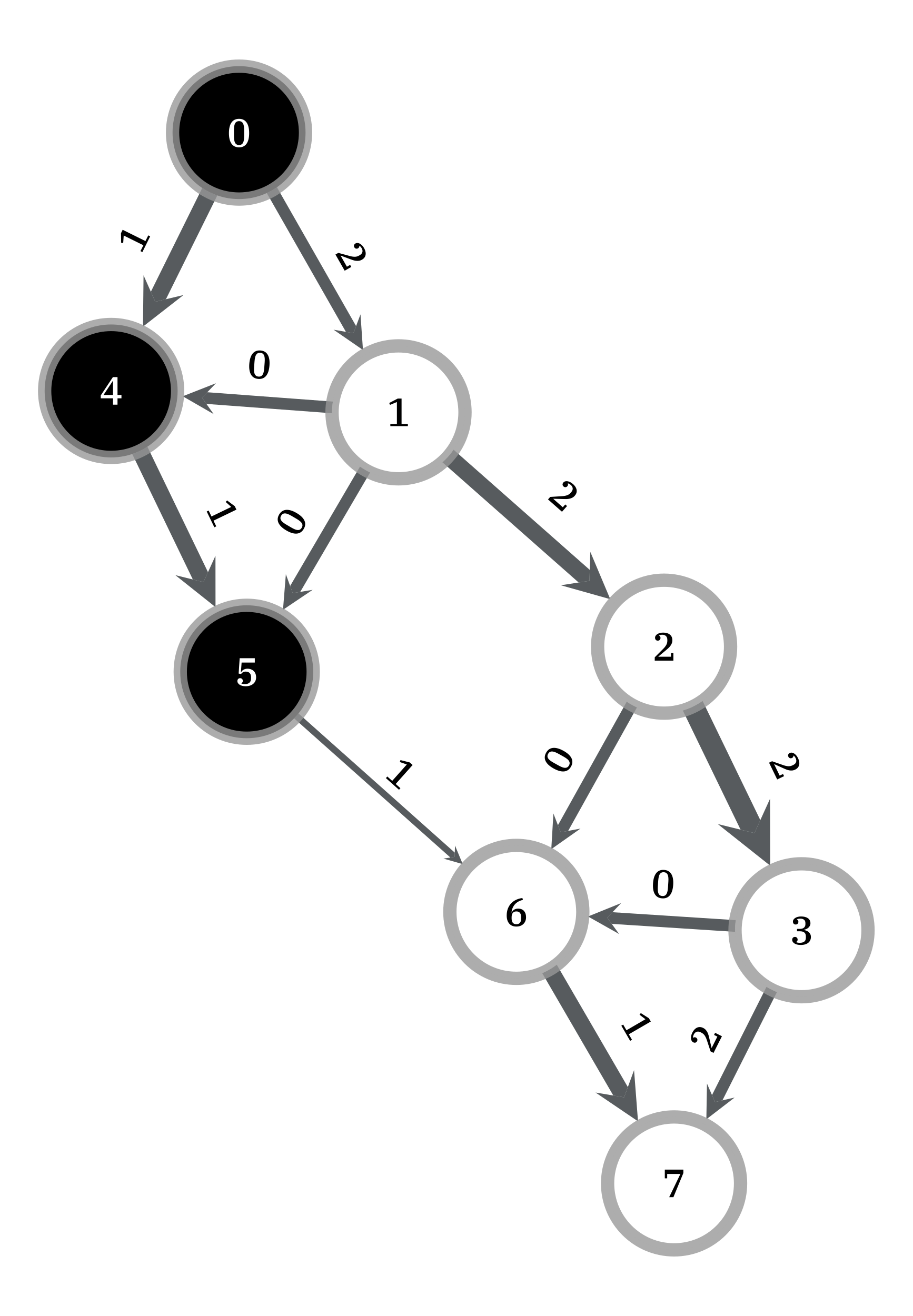
Edge flows obtained with the Boykov-Kolmogorov algorithm. The source and target are labeled
0and7, respectively. The edge capacities are represented by the edge width, and the maximum flow by the edge labels. Vertices of the same color are on the same side the minimum cut.#