boykov_kolmogorov_max_flow#
- graph_tool.flow.boykov_kolmogorov_max_flow(g, source, target, capacity, residual=None)[source]#
Calculate maximum flow on the graph with the Boykov-Kolmogorov algorithm.
- Parameters:
- g
Graph Graph to be used.
- sourceVertex
The source vertex.
- targetVertex
The target (or “sink”) vertex.
- capacity
EdgePropertyMap Edge property map with the edge capacities.
- residual
EdgePropertyMap(optional, default: none) Edge property map where the residuals should be stored.
- g
- Returns:
- residual
EdgePropertyMap Edge property map with the residual capacities (capacity - flow).
- residual
Notes
The algorithm is defined in [kolmogorov-graph-2003] and [boykov-experimental-2004]. The worst case complexity is \(O(EV^2|C|)\), where \(|C|\) is the minimum cut (but typically performs much better).
For a more detailed description, see [boost-kolmogorov].
References
[kolmogorov-graph-2003]Vladimir Kolmogorov, “Graph Based Algorithms for Scene Reconstruction from Two or More Views”, PhD thesis, Cornell University, September 2003.
[boykov-experimental-2004]Yuri Boykov and Vladimir Kolmogorov, “An Experimental Comparison of Min-Cut/Max-Flow Algorithms for Energy Minimization in Vision”, IEEE Transactions on Pattern Analysis and Machine Intelligence, vol. 26, no. 9, pp. 1124-1137, Sept. 2004. DOI: 10.1109/TPAMI.2004.60 [sci-hub, @tor]
Examples
>>> g = gt.load_graph("flow-example.xml.gz")
>>> cap = g.edge_properties["cap"]
>>> src, tgt = g.vertex(0), g.vertex(1)
>>> res = gt.boykov_kolmogorov_max_flow(g, src, tgt, cap)
>>> res.a = cap.a - res.a  # the actual flow
>>> max_flow = sum(res[e] for e in tgt.in_edges())
>>> print(max_flow)
44.8905957841...
>>> pos = g.vertex_properties["pos"]
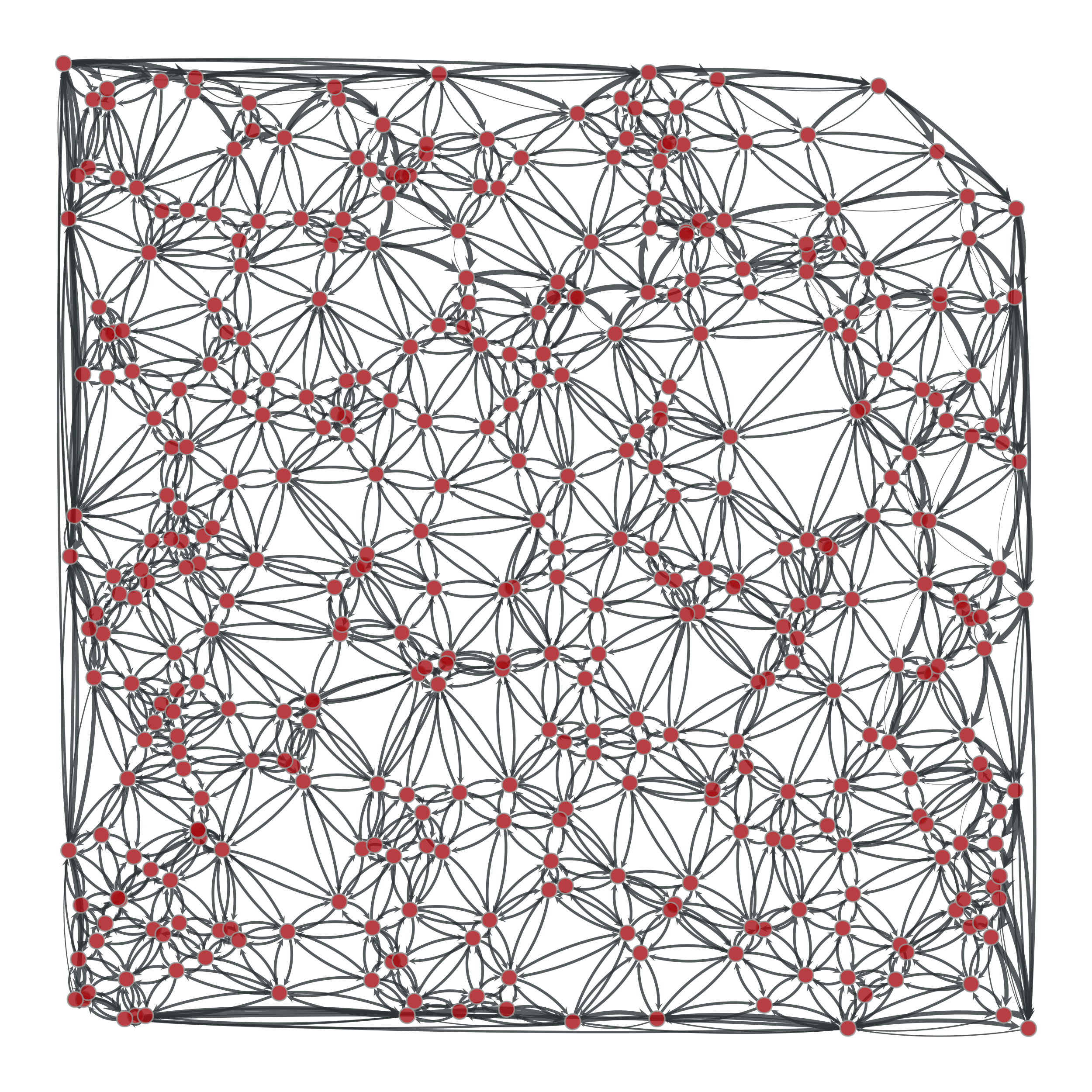
>>> gt.graph_draw(g, pos=pos, edge_pen_width=gt.prop_to_size(res, mi=0, ma=3, power=1), output="example-kolmogorov.pdf")
<...>

Edge flows obtained with the Boykov-Kolmogorov algorithm. The source and target are on the upper left and lower right corners, respectively. The edge flows are represented by the edge width.#