closeness#
- graph_tool.centrality.closeness(g, weight=None, source=None, vprop=None, norm=True, harmonic=False)[source]#
Calculate the closeness centrality for each vertex.
- Parameters:
- g
Graph Graph to be used.
- weight
EdgePropertyMap, optional (default: None) Edge property map corresponding to the weight value of each edge.
- source
Vertex, optional (default:None) If specified, the centrality is computed for this vertex alone.
- vprop
VertexPropertyMap, optional (default:None) Vertex property map to store the vertex centrality values.
- normbool, optional (default:
True) Whether or not the centrality values should be normalized.
- harmonicbool, optional (default:
False) If true, the sum of the inverse of the distances will be computed, instead of the inverse of the sum.
- g
- Returns:
- vertex_closeness
VertexPropertyMap A vertex property map with the vertex closeness values.
- vertex_closeness
See also
central_point_dominancecentral point dominance of the graph
pagerankPageRank centrality
eigentrusteigentrust centrality
eigenvectoreigenvector centrality
hitsauthority and hub centralities
trust_transitivitypervasive trust transitivity
Notes
The closeness centrality of a vertex \(i\) is defined as,
\[c_i = \frac{1}{\sum_j d_{ij}}\]where \(d_{ij}\) is the (possibly directed and/or weighted) distance from \(i\) to \(j\). In case there is no path between the two vertices, here the distance is taken to be zero.
If
harmonic == True, the definition becomes\[c_i = \sum_j\frac{1}{d_{ij}},\]but now, in case there is no path between the two vertices, we take \(d_{ij} \to\infty\) such that \(1/d_{ij}=0\).
If
norm == True, the values of \(c_i\) are normalized by \(n_i-1\) where \(n_i\) is the size of the (out-) component of \(i\). Ifharmonic == True, they are instead simply normalized by \(V-1\).The algorithm complexity of \(O(V(V + E))\) for unweighted graphs and \(O(V(V+E) \log V)\) for weighted graphs. If the option
sourceis specified, this drops to \(O(V + E)\) and \(O((V+E)\log V)\) respectively.Parallel implementation.
If enabled during compilation, this algorithm will run in parallel using OpenMP. See the parallel algorithms section for information about how to control several aspects of parallelization.
References
[closeness-wikipedia][opsahl-node-2010]Opsahl, T., Agneessens, F., Skvoretz, J., “Node centrality in weighted networks: Generalizing degree and shortest paths”. Social Networks 32, 245-251, 2010 DOI: 10.1016/j.socnet.2010.03.006 [sci-hub, @tor]
[adamic-polblogs]L. A. Adamic and N. Glance, “The political blogosphere and the 2004 US Election”, in Proceedings of the WWW-2005 Workshop on the Weblogging Ecosystem (2005). DOI: 10.1145/1134271.1134277 [sci-hub, @tor]
Examples
>>> g = gt.collection.data["polblogs"]
>>> g = gt.GraphView(g, vfilt=gt.label_largest_component(g))
>>> c = gt.closeness(g)
>>> gt.graph_draw(g, pos=g.vp["pos"], vertex_fill_color=c,
...               vertex_size=gt.prop_to_size(c, mi=5, ma=15),
...               vcmap=matplotlib.cm.gist_heat,
...               vorder=c, output="polblogs_closeness.pdf")
<...>
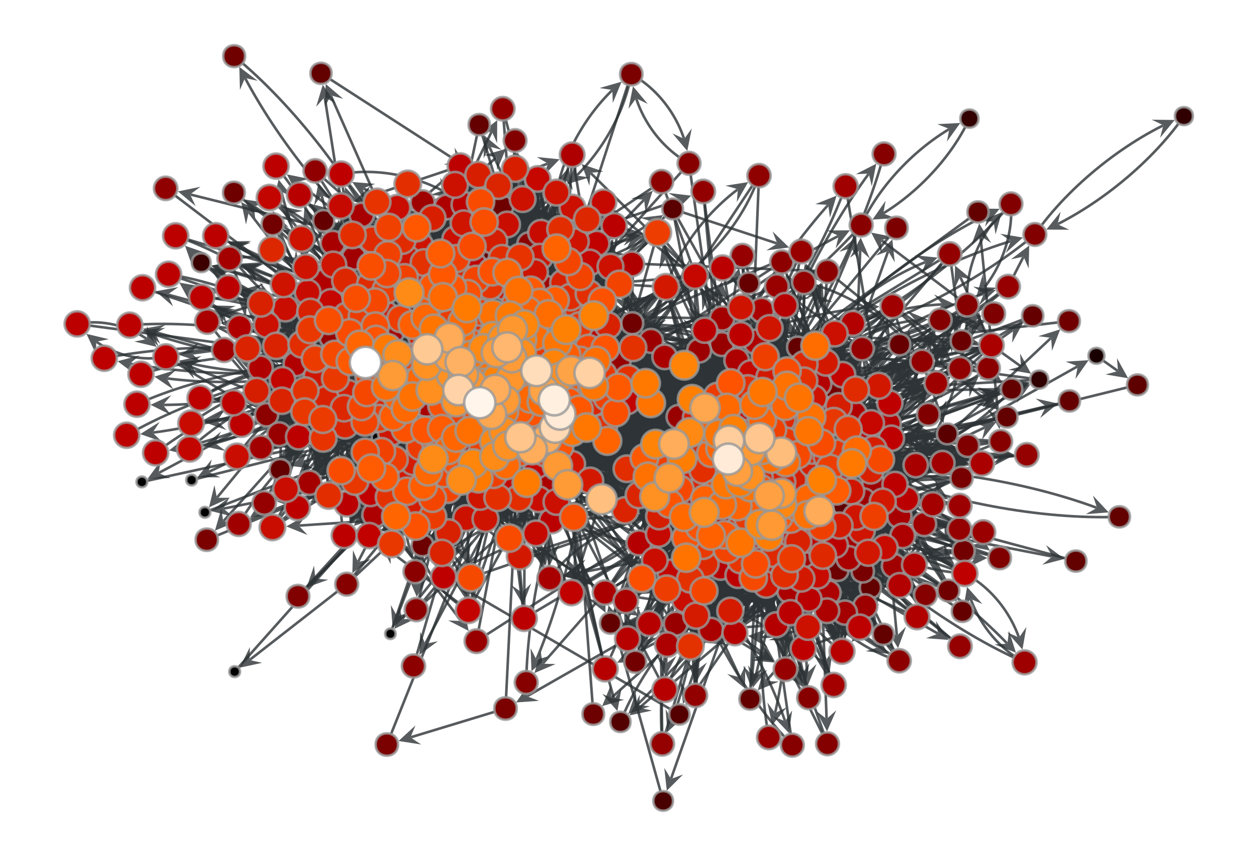
Closeness values of the a political blogs network of [adamic-polblogs].#