Quick start guide#
The graph_tool module provides a Graph class
and several algorithms that operate on it. The internals of this class,
and of most algorithms, are written in C++ for performance, using the
Boost Graph Library.
The module must be of course imported before it can be used. The package is subdivided into several sub-modules. To import everything from all of them, one can do:
>>> from graph_tool.all import *
In the following, it will always be assumed that the previous line was run.
Creating graphs#
An empty graph can be created by instantiating a Graph
class:
>>> g = Graph()
By default, newly created graphs are always directed. To construct undirected
graphs, one must pass a value to the directed parameter:
>>> ug = Graph(directed=False)
A graph can always be switched on-the-fly from directed to undirected
(and vice versa), with the set_directed()
method. The “directedness” of the graph can be queried with the
is_directed() method:
>>> ug = Graph()
>>> ug.set_directed(False)
>>> assert ug.is_directed() == False
Once a graph is created, it can be populated with vertices and edges. A
vertex can be added with the add_vertex()
method, which returns an instance of a Vertex
class, also called a vertex descriptor. For instance, the following
code creates two vertices, and returns vertex descriptors stored in the
variables v1 and v2.
>>> v1 = g.add_vertex()
>>> v2 = g.add_vertex()
Edges can be added in an analogous manner, by calling the
add_edge() method, which returns an edge
descriptor (an instance of the Edge class):
>>> e = g.add_edge(v1, v2)
The above code creates a directed edge from v1 to v2.
A graph can also be created by providing another graph, in which case the entire graph (and its internal property maps, see Property maps) is copied:
>>> g2 = Graph(g) # g2 is a copy of g
Above, g2 is a “deep” copy of g, i.e. any modification of
g2 will not affect g.
Note
Graph visualization in graph-tool can be interactive! When the output
parameter of graph_draw() is omitted, instead of saving
to a file, the function opens an interactive window. From there, the user can
zoom in or out, rotate the graph, select and move individual nodes or node
selections. See GraphWidget() for documentation on the
interactive interface.
If you are using a Jupyter notebook, the graphs
are drawn inline if output is omitted. If an interactive window is
desired instead, the option inline = False should be passed.
We can visualize the graph we created so far with the
graph_draw() function.
>>> graph_draw(g, vertex_text=g.vertex_index, output="two-nodes.svg")
<...>

A simple directed graph with two vertices and one edge, created by the commands above.#
We can add attributes to the nodes and edges of our graph via property maps. For example, suppose we want to add an edge weight and
node color to our graph we have first to create two PropertyMap
objects as such:
>>> eweight = g.new_ep("double")    # creates an EdgePropertyMap of type double
>>> vcolor = g.new_vp("string")     # creates a VertexPropertyMap of type string
And now we set their values for each vertex and edge:
>>> eweight[e] = 25.3
>>> vcolor[v1] = "#1c71d8"
>>> vcolor[v2] = "#2ec27e"
Property maps can then be used in many graph-tool functions to set node
and edge properties, for example:
>>> graph_draw(g, vertex_text=g.vertex_index, vertex_fill_color=vcolor,
...            edge_pen_width=eweight, output="two-nodes-color.svg")
<...>

The same graph as before, but with edge width and node color specified by property maps.#
Property maps are discussed in more detail in the section Property maps below.
Adding many edges and vertices at once#
Note
The vertex values passed to the constructor need to be integers per default,
but arbitrary objects can be passed as well if the option hashed = True
is passed. In this case, the mapping of vertex descriptors to
vertex ids is obtained via an internal
VertexPropertyMap called "ids". E.g. in the
example above we have
>>> print(g.vp.ids[0])
foo
See Property maps below for more details.
It is also possible to add many edges and vertices at once when the graph is created. For example, it is possible to construct graphs directly from a list of edges, e.g.
>>> g = Graph([('foo', 'bar'), ('gnu', 'gnat')], hashed=True)
which is just a convenience shortcut to creating an empty graph and calling
add_edge_list() afterward, as we will discuss below.
Edge properties can also be initialized together with the edges by using
tuples (source, target, property_1, property_2, ...), e.g.
>>> g = Graph([('foo', 'bar', .5, 1), ('gnu', 'gnat', .78, 2)], hashed=True,
...           eprops=[('weight', 'double'), ('time', 'int')])
The eprops parameter lists the name and value types of the properties, which
are used to create internal property maps with the value encountered (see
Property maps below for more details).
It is possible also to pass an adjacency list to construct a graph, which is a dictionary of out-neighbors for every vertex key:
>>> g = Graph({0: [2, 3], 1: [4], 3: [4, 5], 6: []})
We can also easily construct graphs from adjacency matrices. They need only to
be converted to a sparse scipy matrix (i.e. a subclass of
scipy.sparse.sparray or scipy.sparse.spmatrix) and passed to
the constructor, e.g.:
>>> m = np.array([[0, 1, 0],
...               [0, 0, 1],
...               [0, 1, 0]])
>>> g = Graph(scipy.sparse.lil_matrix(m))
The nonzero entries of the matrix are stored as an edge property map named
"weight" (see Property maps below for more details), e.g.
>>> m = np.array([[0, 1.2, 0],
...               [0, 0, 10],
...               [0, 7, 0]])
>>> g = Graph(scipy.sparse.lil_matrix(m))
>>> print(g.ep.weight.a)
[ 1.2  7.  10. ]
For undirected graphs (i.e. the option directed = False is given) only the
upper triangular portion of the passed matrix will be considered, and the
remaining entries will be ignored.
We can also add many edges at once after the graph has been created using the
add_edge_list() method. It accepts any iterable of
(source, target) pairs, and automatically adds any new vertex seen:
>>> g.add_edge_list([(0, 1), (2, 3)])
Note
As above, if hashed = True is passed, the function
add_edge_list() returns a
VertexPropertyMap object that maps vertex descriptors to
their id values in the list. See Property maps below.
The vertex values passed to add_edge_list() need to be
integers per default, but arbitrary objects can be passed as well if the
option hashed = True is passed, e.g. for string values:
>>> g.add_edge_list([('foo', 'bar'), ('gnu', 'gnat')], hashed=True,
...                 hash_type="string")
<...>
or for arbitrary (hashable) Python objects:
>>> g.add_edge_list([((2, 3), 'foo'), (3, 42.3)], hashed=True,
...                 hash_type="object")
<...>
Manipulating graphs#
With vertex and edge descriptors at hand, one can examine and manipulate
the graph in an arbitrary manner. For instance, in order to obtain the
out-degree of a vertex, we can simply call the
out_degree() method:
>>> g = Graph()
>>> v1 = g.add_vertex()
>>> v2 = g.add_vertex()
>>> e = g.add_edge(v1, v2)
>>> print(v1.out_degree())
1
Note
For undirected graphs, the “out-degree” is synonym for degree, and in this case the in-degree of a vertex is always zero.
Analogously, we could have used the in_degree()
method to query the in-degree.
Edge descriptors have two useful methods, source()
and target(), which return the source and target
vertex of an edge, respectively.
>>> print(e.source(), e.target())
0 1
We can also directly convert an edge to a tuple of vertices, to the same effect:
>>> u, v = e
>>> print(u, v)
0 1
The add_vertex() method also accepts an optional
parameter which specifies the number of additional vertices to create. If this
value is greater than 1, it returns an iterator on the added vertex descriptors:
>>> vlist = g.add_vertex(10)
>>> print(len(list(vlist)))
10
Each vertex in a graph has a unique index, which is *always* between
\(0\) and \(N-1\), where \(N\) is the number of
vertices. This index can be obtained by using the
vertex_index attribute of the graph (which is
a property map, see Property maps), or by converting the
vertex descriptor to an int.
>>> v = g.add_vertex()
>>> print(g.vertex_index[v])
12
>>> print(int(v))
12
Edges and vertices can also be removed at any time with the
remove_vertex() and remove_edge() methods,
>>> g.remove_edge(e)                               # e no longer exists
>>> g.remove_vertex(v2)                # the second vertex is also gone
When removing edges, it is important to keep in mind some performance considerations:
Warning
Because of the contiguous indexing, removing a vertex with an index smaller
than \(N-1\) will invalidate either the last (fast == True) or
all (fast == False) descriptors pointing to vertices with higher
index.
As a consequence, if more than one vertex is to be removed at a given time, they should always be removed in decreasing index order:
# 'vs' is a list of
# vertex descriptors
vs = sorted(vs)
vs = reversed(vs)
for v in vs:
    g.remove_vertex(v)
Alternatively (and preferably), a list (or any iterable) may be
passed directly as the vertex parameter of the
remove_vertex() function, and the above is
performed internally (in C++).
Note that property map values (see Property maps) are unaffected by the index changes due to vertex removal, as they are modified accordingly by the library.
Note
Removing a vertex is typically an \(O(N)\) operation. The
vertices are internally stored in a STL vector, so removing an
element somewhere in the middle of the list requires the shifting of
the rest of the list. Thus, fast \(O(1)\) removals are only
possible if one can guarantee that only vertices in the end of the
list are removed (the ones last added to the graph), or if the
relative vertex ordering is invalidated. The latter behavior can be
achieved by passing the option fast = True, to
remove_vertex(), which causes the vertex
being deleted to be ‘swapped’ with the last vertex (i.e. with the
largest index), which, in turn, will inherit the index of the vertex
being deleted.
Removing an edge is an \(O(k_{s} + k_{t})\) operation, where
\(k_{s}\) is the out-degree of the source vertex, and
\(k_{t}\) is the in-degree of the target vertex. This can be made
faster by setting set_fast_edge_removal() to
True, in which case it becomes \(O(1)\), at the expense of
additional data of size \(O(E)\).
No edge descriptors are ever invalidated after edge removal, with the exception of the edge itself that is being removed.
Since vertices are uniquely identifiable by their indices, there is no
need to keep the vertex descriptor lying around to access them at a
later point. If we know its index, we can obtain the descriptor of a
vertex with a given index using the vertex()
method,
>>> v = g.vertex(8)
which takes an index, and returns a vertex descriptor. Edges cannot be
directly obtained by its index, but if the source and target vertices of
a given edge are known, it can be retrieved with the
edge() method
>>> g.add_edge(g.vertex(2), g.vertex(3))
<...>
>>> e = g.edge(2, 3)
Another way to obtain edge or vertex descriptors is to iterate through them, as described in section Iterating over vertices and edges. This is in fact the most useful way of obtaining vertex and edge descriptors.
Like vertices, edges also have unique indices, which are given by the
edge_index property:
>>> e = g.add_edge(g.vertex(0), g.vertex(1))
>>> print(g.edge_index[e])
1
Differently from vertices, edge indices do not necessarily conform to any specific range. If no edges are ever removed, the indices will be in the range \([0, E-1]\), where \(E\) is the number of edges, and edges added earlier have lower indices. However if an edge is removed, its index will be “vacant”, and the remaining indices will be left unmodified, and thus will not all lie in the range \([0, E-1]\). If a new edge is added, it will reuse old indices, in an increasing order.
Iterating over vertices and edges#
Algorithms must often iterate through vertices, edges, out-edges of a
vertex, etc. The Graph and
Vertex classes provide different types of iterators
for doing so. The iterators always point to edge or vertex descriptors.
Iterating over all vertices or edges#
In order to iterate through all the vertices or edges of a graph, the
vertices() and edges()
methods should be used:
for v in g.vertices():
    print(v)
for e in g.edges():
    print(e)
The code above will print the vertices and edges of the graph in the order they are found.
Iterating over the neighborhood of a vertex#
Warning
You should never remove vertex or edge descriptors when iterating over them, since this invalidates the iterators. If you plan to remove vertices or edges during iteration, you must first store them somewhere (such as in a list) and remove them only after no iterator is being used. Removal during iteration will cause bad things to happen.
The out- and in-edges of a vertex, as well as the out- and in-neighbors can be
iterated through with the out_edges(),
in_edges(), out_neighbors()
and in_neighbors() methods, respectively.
for v in g.vertices():
   for e in v.out_edges():
       print(e)
   for w in v.out_neighbors():
       print(w)

   # the edge and neighbors order always match
   for e, w in zip(v.out_edges(), v.out_neighbors()):
       assert e.target() == w
The code above will print the out-edges and out-neighbors of all vertices in the graph.
Example analysis: an online social network#
Let us consider an online social network of facebook users, available from the
Netzschleuder network repository. We can load it
in graph-tool via the graph_tool.collection.ns interface:
>>> g = collection.ns["ego_social/facebook_combined"]
We can quickly inspect the structure of the network by visualizing it:
>>> graph_draw(g, g.vp._pos, output="facebook.pdf")
<...>
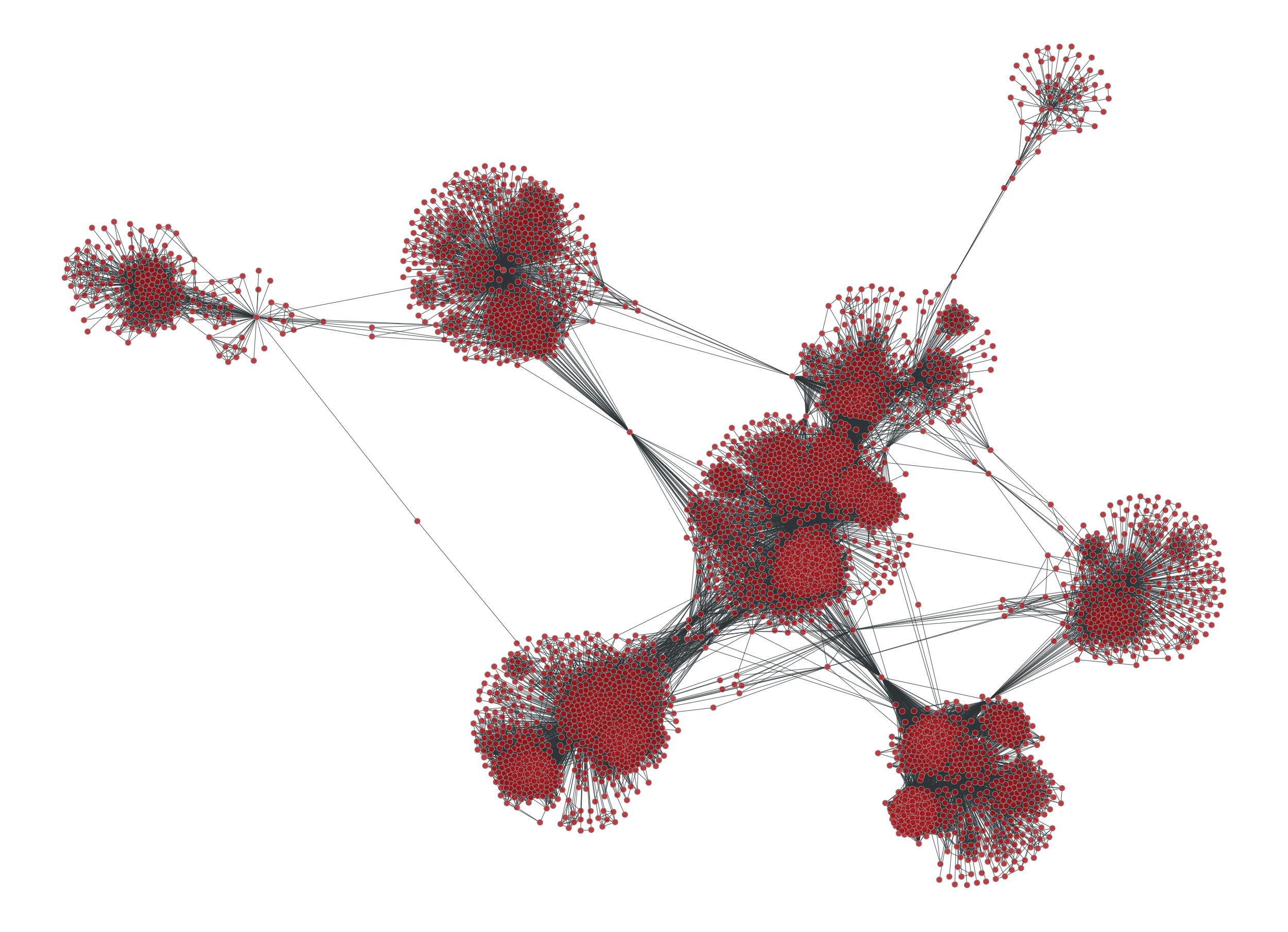
Network of friendships among users on Facebook.#
Note
A SBM provides a statistically principled method to cluster the nodes of a
network according to their latent mixing patterns. graph-tool provides
extensive support for this kind of analysis, as detailed in a dedicated HOWTO.
This methodology overcomes some serious limitations of outdated approaches, such as modularity maximization, which should in general be avoided.
This network seems to be composed of many communities with homophilic patterns.
We can identify them reliably by inferring a stochastic block model (SBM),
achieved by calling minimize_blockmodel_dl():
>>> state = minimize_blockmodel_dl(g)
This returns a BlockState object. We can
visualize the results with:
>>> state.draw(pos=g.vp._pos, output="facebook-sbm.pdf")
<...>
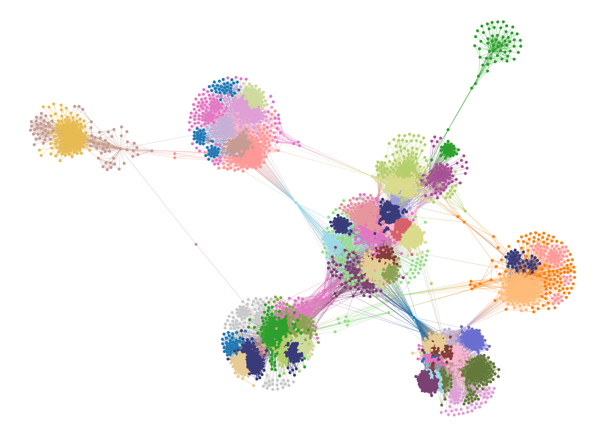
Groups of nodes identified by fitting a SBM to the facebook frendship data.#
Note
The algorithm to compute betweenness centrality has a quadratic complexity on
the number of nodes of the network, so it can become slow as it becomes large.
However in graph-tool it is implemented in parallel, affording us more
performance. For the network being considered, it finishes in under a second
with a modern laptop.
We might want to identify the nodes and edges that act as “bridges” between
these communities. We can do so by computing the betweenness centrality, obtained via
betweenness():
>>> vb, eb = betweenness(g)
This returns an vertex and edge property map with the respective betweenness values. We can visualize them with:
Tip
The function prop_to_size() provides a convenient way
to transformation the property map values to ranges more appropriate for
sizes in graph_draw(). See also
Transformations.
>>> graph_draw(g, g.vp._pos, vertex_fill_color=prop_to_size(vb, 0, 1, power=.1),
...            vertex_size=prop_to_size(vb, 3, 12, power=.2), vorder=vb,
...            output="facebook-bt.pdf")
<...>
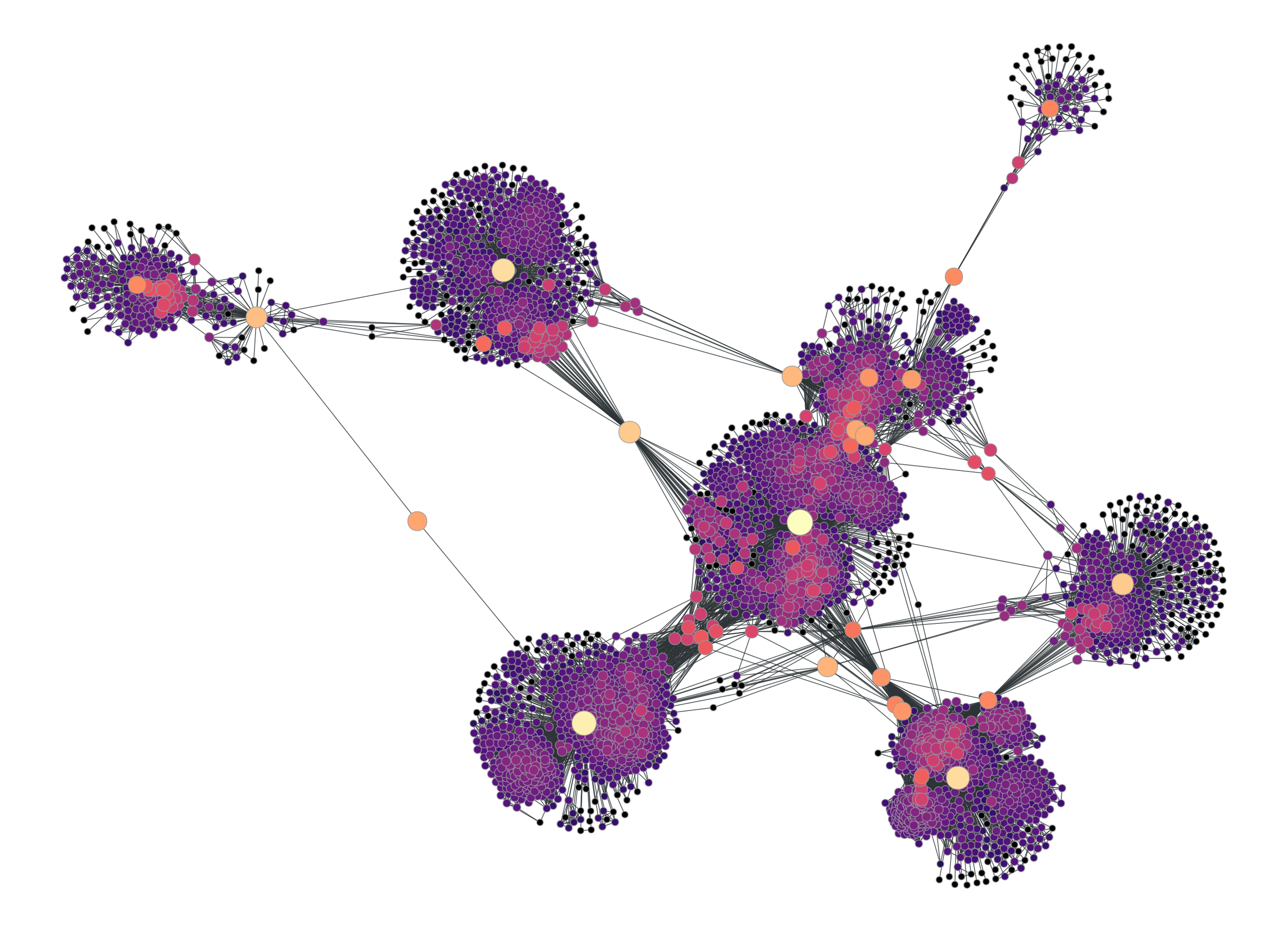
The node betweeness values correspond to the color and size of the nodes.#
Property maps#
Property maps are a way of associating additional information to the
vertices, edges, or to the graph itself. There are thus three types of
property maps: vertex, edge, and graph. They are handled by the
classes VertexPropertyMap,
EdgePropertyMap, and
GraphPropertyMap. Each created property map has an
associated value type, which must be chosen from the predefined set:
Type name |
Alias |
|---|---|
|
|
|
|
|
|
|
|
|
|
|
|
|
|
|
|
|
|
|
|
|
|
|
|
|
|
|
|
|
|
New property maps can be created for a given graph by calling one of the
methods new_vertex_property() (alias
new_vp()),
new_edge_property() (alias
new_ep()), or
new_graph_property() (alias
new_gp()), for each map type. The values are
then accessed by vertex or edge descriptors, or the graph itself, as
such:
from numpy.random import randint

g = Graph()
g.add_vertex(100)

# insert some random links
for s, t in zip(randint(0, 100, 100), randint(0, 100, 100)):
    g.add_edge(g.vertex(s), g.vertex(t))

vprop = g.new_vertex_property("double")              # Double-precision floating point
v = g.vertex(10)
vprop[v] = 3.1416

vprop2 = g.new_vertex_property("vector<int>")        # Vector of ints
v = g.vertex(40)
vprop2[v] = [1, 3, 42, 54]

eprop = g.new_edge_property("object")                # Arbitrary Python object.
e = g.edges().next()
eprop[e] = {"foo": "bar", "gnu": 42}                 # In this case, a dict.

gprop = g.new_graph_property("bool")                 # Boolean
gprop[g] = True
It is possible also to access vertex property maps directly by vertex indices:
>>> print(vprop[10])
3.1416
Warning
The following lines are equivalent:
eprop[(30, 40)]
eprop[g.edge(30, 40)]
Which means that indexing via (source, target) pairs is slower than via edge
descriptors, since the function edge() needs to be
called first.
And likewise we can access edge descriptors via (source, target) pairs:
>>> g.add_edge(30, 40)
<...>
>>> eprop[(30, 40)] = "gnat"
We can also iterate through the property map values directly, i.e.
>>> print(list(vprop)[:10])
[0.0, 0.0, 0.0, 0.0, 0.0, 0.0, 0.0, 0.0, 0.0, 0.0]
Property maps with scalar value types can also be accessed as a
numpy.ndarray, with the
get_array() method, or the
a attribute, e.g.,
from numpy.random import random

# this assigns random values to the vertex properties
vprop.get_array()[:] = random(g.num_vertices())

# or more conveniently (this is equivalent to the above)
vprop.a = random(g.num_vertices())
Array interface for filtered graphs
For filtered graphs (see Graph filtering below), it’s possible
to get arrays that only point to the nodes and edges that are not filtered
out via the fa and
ma attributes instead.
Transformations#
We usually want to apply transformations to the values of property maps. This
can be achieved via iteration (see Iterating over vertices and edges), but since this is a
such a common operation, there’s a more convenient way to do this via the
transform() method (or is shorter alias
t()), which takes a function and returns a
copy of the property map with the function applied to its values:
from numpy import abs
from numpy.random import random

# Vertex property map with random values in the range [-.5, .5]
rand = g.new_vp("double", vals=random(g.num_vertices()) - .5)

# The following returns a copy of `rand` but containing only the absolute values
m = rand.t(abs)
Tip
Transformations are particularly useful to pass temporary properties to functions, e.g.
erand = g.new_ep("double", vals=random(g.num_edges()) - .5)
pos = sfdp_layout(g, eweight=erand.t(abs))
Internal property maps#
Any created property map can be made “internal” to the corresponding
graph. This means that it will be copied and saved to a file together
with the graph. Properties are internalized by including them in the
graph’s dictionary-like attributes
vertex_properties,
edge_properties or
graph_properties (or their aliases,
vp, ep or
gp, respectively). When inserted in the graph,
the property maps must have an unique name (between those of the same
type):
>>> eprop = g.new_edge_property("string")
>>> g.ep["some name"] = eprop
>>> g.list_properties()
some name      (edge)    (type: string)
Internal graph property maps behave slightly differently. Instead of returning the property map object, the value itself is returned from the dictionaries:
>>> gprop = g.new_graph_property("int")
>>> g.gp["foo"] = gprop                 # this sets the actual property map
>>> g.gp["foo"] = 42                    # this sets its value
>>> print(g.gp["foo"])
42
>>> del g.gp["foo"]                     # the property map entry is deleted from the dictionary
For convenience, the internal property maps can also be accessed via attributes:
>>> vprop = g.new_vertex_property("double")
>>> g.vp.foo = vprop                    # equivalent to g.vp["foo"] = vprop
>>> v = g.vertex(0)
>>> g.vp.foo[v] = 3.14
>>> print(g.vp.foo[v])
3.14
Graph I/O#
Graphs can be saved and loaded in four formats: graphml, dot, gml
and a custom binary format gt (see The gt file format).
Warning
The binary format gt and the text-based graphml are the
preferred formats, since they are by far the most complete. Both
these formats are equally complete, but the gt format is faster
and requires less storage.
The dot and gml formats are fully supported, but since they
contain no precise type information, all properties are read as
strings (or also as double, in the case of gml), and must be
converted by hand to the desired type. Therefore you should always
use either gt or graphml, since they implement an exact
bit-for-bit representation of all supported Property maps
types, except when interfacing with other software, or existing
data, which uses dot or gml.
Note
Graph classes can also be pickled with the pickle module.
A graph can be saved or loaded to a file with the save
and load methods, which take either a file name or a
file-like object. A graph can also be loaded from disc with the
load_graph() function, as such:
g = Graph()
#  ... fill the graph ...
g.save("my_graph.gt.gz")
g2 = load_graph("my_graph.gt.gz")
# g and g2 should be identical copies of each other
Graph filtering#
Note
It is important to emphasize that the filtering functionality does not add any performance overhead when the graph is not being filtered. In this case, the algorithms run just as fast as if the filtering functionality didn’t exist.
One of the unique features of graph-tool is the “on-the-fly” filtering of
edges and/or vertices. Filtering means the temporary masking of vertices/edges,
which are in fact not really removed, and can be easily recovered.
Ther are two different ways to enable graph filtering: via graph views or inplace filtering, which are covered in the following.
Graph views#
It is often desired to work with filtered and unfiltered graphs
simultaneously, or to temporarily create a filtered version of graph for
some specific task. For these purposes, graph-tool provides a
GraphView class, which represents a filtered “view”
of a graph, and behaves as an independent graph object, which shares the
underlying data with the original graph. Graph views are constructed by
instantiating a GraphView class, and passing a
graph object which is supposed to be filtered, together with the desired
filter parameters. For example, to create a directed view of an undirected graph
g above, one could do:
>>> ug = GraphView(g, directed=True)
>>> ug.is_directed()
True
Graph views also provide a direct and convenient approach to vertex/edge filtering. Let us consider the facebook friendship graph we used before and the betweeness centrality values:
>>> g = collection.ns["ego_social/facebook_combined"]
>>> vb, eb = betweenness(g)
Let us suppose we would like to see how the graph would look like if some of the
edges with higher betweeness values were removed. We can do this by a
GraphView object and passing the efilt paramter:
>>> u = GraphView(g, efilt=eb.fa < 1e-6)
Note
GraphView objects behave exactly like regular
Graph objects. In fact,
GraphView is a subclass of
Graph. The only difference is that a
GraphView object shares its internal data with
its parent Graph class. Therefore, if the
original Graph object is modified, this
modification will be reflected immediately in the
GraphView object, and vice versa.
Since GraphView is a derived class from
Graph, and its instances are accepted as regular graphs
by every function of the library. Graph views are “first class citizens” in
graph-tool.
If we visualize the graph we can see it now has been broken up in many components:
>>> graph_draw(u, pos=g.vp._pos, output="facebook-filtered.pdf")
<...>
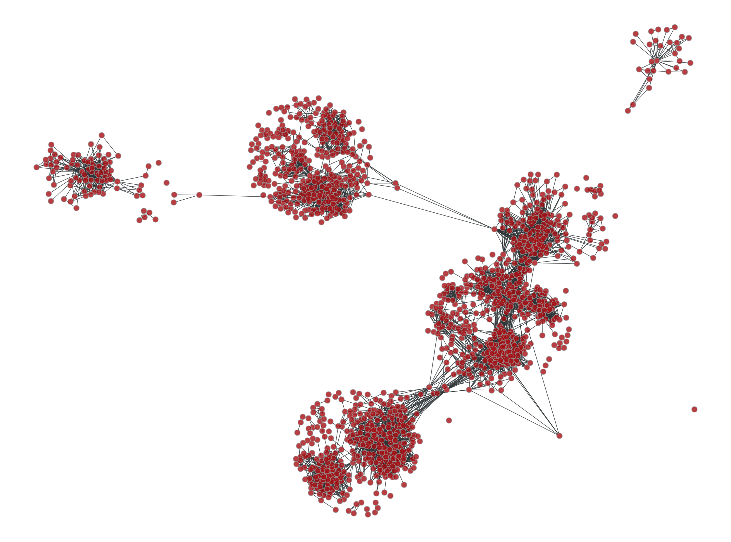
Facebook friendship network with edges with a betweeness centrality value above \(10^{-6}\) filtered out.#
Note however that no copy of the original graph was done, and no edge has been
in fact removed. If we inspect the original graph g in the example above, it
will be intact.
In the example above, we passed a boolean array as the efilt, but we could
have passed also a boolean property map, a function that takes an edge as
single parameter, and returns True if the edge should be kept and
False otherwise. For instance, the above could be equivalently achieved as:
>>> u = GraphView(g, efilt=lambda e: eb[e] < 1e-6)
But note however that would be slower, since it would involve one function call per edge in the graph.
Vertices can also be filtered in an entirerly analogous fashion using the
vfilt paramter.
Composing graph views#
Since graph views behave like regular graphs, one can just as easily create
graph views of graph views. This provides a convenient way of composing
filters. For instance, suppose we wanto to isolate the minimum spanning tree of all
vertices of agraph above which have a degree larger than four:
>>> g, pos = triangulation(random((500, 2)) * 4, type="delaunay")
>>> u = GraphView(g, vfilt=lambda v: v.out_degree() > 4)
>>> tree = min_spanning_tree(u)
>>> u = GraphView(u, efilt=tree)
The resulting graph view can be used and visualized as normal:
>>> bv, be = betweenness(u)
>>> be.a /= be.a.max() / 5
>>> graph_draw(u, pos=pos, vertex_fill_color=bv,
...            edge_pen_width=be, output="mst-view.svg")
<...>

A composed view, obtained as the minimum spanning tree of all vertices in the graph which have a degree larger than four. The edge thickness indicates the betweeness values, as well as the node colors.#
In-place graph filtering#
It is possible also to filter graphs “in-place”, i.e. without creating an
additional object. To achieve this, vertices or edges which are to be filtered
should be marked with a PropertyMap with value type
bool, and then set with set_vertex_filter() or
set_edge_filter() methods. Vertex or edges with value
“1” are kept in the graphs, and those with value “0” are filtered out. All
manipulation functions and algorithms will work as if the marked edges or
vertices were removed from the graph, with minimum overhead.
For example, to reproduce the same example as before for the facebook graph we could have done:
>>> g = collection.ns["ego_social/facebook_combined"]
>>> vb, eb = betweenness(g)
>>> mask = g.new_ep("bool", vals = eb.fa < 1e-5)
>>> g.set_edge_filter(mask)
The mask property map has a bool type, with value 1 if the edge belongs to
the tree, and 0 otherwise.
Everything should work transparently on the filtered graph, simply as if the masked edges were removed.
The original graph can be recovered by setting the edge filter to None.
g.set_edge_filter(None)
Everything works in analogous fashion with vertex filtering.
Additionally, the graph can also have its edges reversed with the
set_reversed() method. This is also an \(O(1)\)
operation, which does not really modify the graph.
As mentioned previously, the directedness of the graph can also be changed
“on-the-fly” with the set_directed() method.
Advanced iteration#
Faster iteration over vertices and edges without descriptors#
The mode of iteration considered above is convenient, but
requires the creation of vertex and edge descriptor objects, which incurs a
performance overhead. A faster approach involves the use of the methods
iter_vertices(), iter_edges(),
iter_out_edges(),
iter_in_edges(),
iter_all_edges(),
iter_out_neighbors(),
iter_in_neighbors(),
iter_all_neighbors(), which return vertex indices and
pairs thereof, instead of descriptors objects, to specify vertex and edges,
respectively.
For example, for the graph:
g = Graph([(0, 1), (2, 3), (2, 4)])
we have
for v in g.iter_vertices():
    print(v)
for e in g.iter_edges():
    print(e)
which yields
0
1
2
3
4
[0, 1]
[2, 3]
[2, 4]
and likewise for the iteration over the neighborhood of a vertex:
for v in g.iter_vertices():
   for e in g.iter_out_edges(v):
       print(e)
   for w in g.iter_out_neighbors(v):
       print(w)
Even faster, “loopless” iteration over vertices and edges using arrays#
While more convenient, looping over the graph as described in the previous
sections are not quite the most efficient approaches to operate on graphs. This
is because the loops are performed in pure Python, thus undermining the
main feature of the library, which is the offloading of loops from Python to
C++. Following the numpy philosophy, graph_tool also provides an
array-based interface that avoids loops in Python. This is done with the
get_vertices(), get_edges(),
get_out_edges(), get_in_edges(),
get_all_edges(),
get_out_neighbors(),
get_in_neighbors(),
get_all_neighbors(),
get_out_degrees(),
get_in_degrees() and
get_total_degrees() methods, which return
numpy.ndarray instances instead of iterators.
For example, using this interface we can get the out-degree of each node via:
print(g.get_out_degrees(g.get_vertices()))
[1 0 2 0 0]
or the sum of the product of the in and out-degrees of the endpoints of each edge with:
edges = g.get_edges()
in_degs = g.get_in_degrees(g.get_vertices())
out_degs = g.get_out_degrees(g.get_vertices())
print((out_degs[edges[:,0]] * in_degs[edges[:,1]]).sum())
5