graph_tool.generation.generate_maxent_sbm

graph_tool.generation.generate_maxent_sbm(b, mrs, out_theta, in_theta=None, directed=False, multigraph=False, self_loops=False)

Generate a random graph by sampling from the maximum-entropy “canonical” stochastic block model.

Parameters:

biterable or numpy.ndarray

Group membership for each node.

mrstwo-dimensional numpy.ndarray or scipy.sparse.spmatrix

Matrix with edge fugacities between groups.

out_thetaiterable or numpy.ndarray

Out-degree fugacities for each node.

in_thetaiterable or numpy.ndarray (optional, default: None)

In-degree fugacities for each node. If not provided, will be identical to out_theta.

directedbool (optional, default: False)

Whether the graph is directed.

multigraphbool (optional, default: False)

Whether parallel edges are allowed.

self_loopsbool (optional, default: False)

Whether self-loops are allowed.

Returns:

gGraph

The generated graph.

See also

solve_sbm_fugacities

Obtain SBM fugacities, given expected degrees and block constraints.

generate_sbm

Generate samples from the Poisson SBM

Notes

The algorithm generates simple or multigraphs according to the degree-corrected maximum-entropy stochastic block model (SBM) [peixoto-latent-2020], which includes the non-degree-corrected SBM as a special case.

The simple graphs are generated with probability:

\[P({\boldsymbol A}|{\boldsymbol \theta},{\boldsymbol \mu},{\boldsymbol b}) = \prod_{i<j} \frac{\left(\theta_i\theta_j\mu_{b_i,b_j}\right)^{A_{ij}}}{1+\theta_i\theta_j\mu_{b_i,b_j}},\]

and the multigraphs with probability:

\[P({\boldsymbol A}|{\boldsymbol \theta},{\boldsymbol \mu},{\boldsymbol b}) = \prod_{i<j} \left(\theta_i\theta_j\mu_{b_i,b_j}\right)^{A_{ij}}(1-\theta_i\theta_j\mu_{b_i,b_j}).\]

In the above, \(\mu_{rs}\) is the edge fugacity between groups \(r\) and \(s\), and \(\theta_i\) is the edge fugacity of node i.

For directed graphs, the probabilities are analogous, i.e.

\[\begin{split}P({\boldsymbol A}|{\boldsymbol \theta}^+,{\boldsymbol \theta}^-,{\boldsymbol \mu},{\boldsymbol b}) &= \prod_{i\ne j} \frac{\left(\theta_i^+\theta_j^-\mu_{b_i,b_j}\right)^{A_{ij}}}{1+\theta_i^+\theta_j^-\mu_{b_i,b_j}} & \quad\text{(simple graphs)},\\ P({\boldsymbol A}|{\boldsymbol \theta}^+,{\boldsymbol \theta}^-,{\boldsymbol \mu},{\boldsymbol b}) &= \prod_{i\ne j} \left(\theta_i^+\theta_j^-\mu_{b_i,b_j}\right)^{A_{ij}}(1-\theta_i^+\theta_j^-\mu_{b_i,b_j}) & \quad\text{(multigraphs)}.\end{split}\]

References

[peixoto-latent-2020]

Tiago P. Peixoto, “Latent Poisson models for networks with heterogeneous density”, DOI: 10.1103/PhysRevE.102.012309 [sci-hub, @tor], arXiv: 2002.07803

Examples

>>> g = gt.collection.data["polblogs"]
>>> g = gt.GraphView(g, vfilt=gt.label_largest_component(g))
>>> g = gt.Graph(g, prune=True)
>>> gt.remove_self_loops(g)
>>> gt.remove_parallel_edges(g)
>>> state = gt.minimize_blockmodel_dl(g)
>>> ers = gt.adjacency(state.get_bg(), state.get_ers()).T
>>> out_degs = g.degree_property_map("out").a
>>> in_degs = g.degree_property_map("in").a
>>> mrs, theta_out, theta_in = gt.solve_sbm_fugacities(state.b.a, ers, out_degs, in_degs)
>>> u = gt.generate_maxent_sbm(state.b.a, mrs, theta_out, theta_in, directed=True)
>>> gt.graph_draw(g, g.vp.pos, output="polblogs-maxent-sbm.pdf")
<...>
>>> gt.graph_draw(u, u.own_property(g.vp.pos), output="polblogs-maxent-sbm-generated.pdf")
<...>

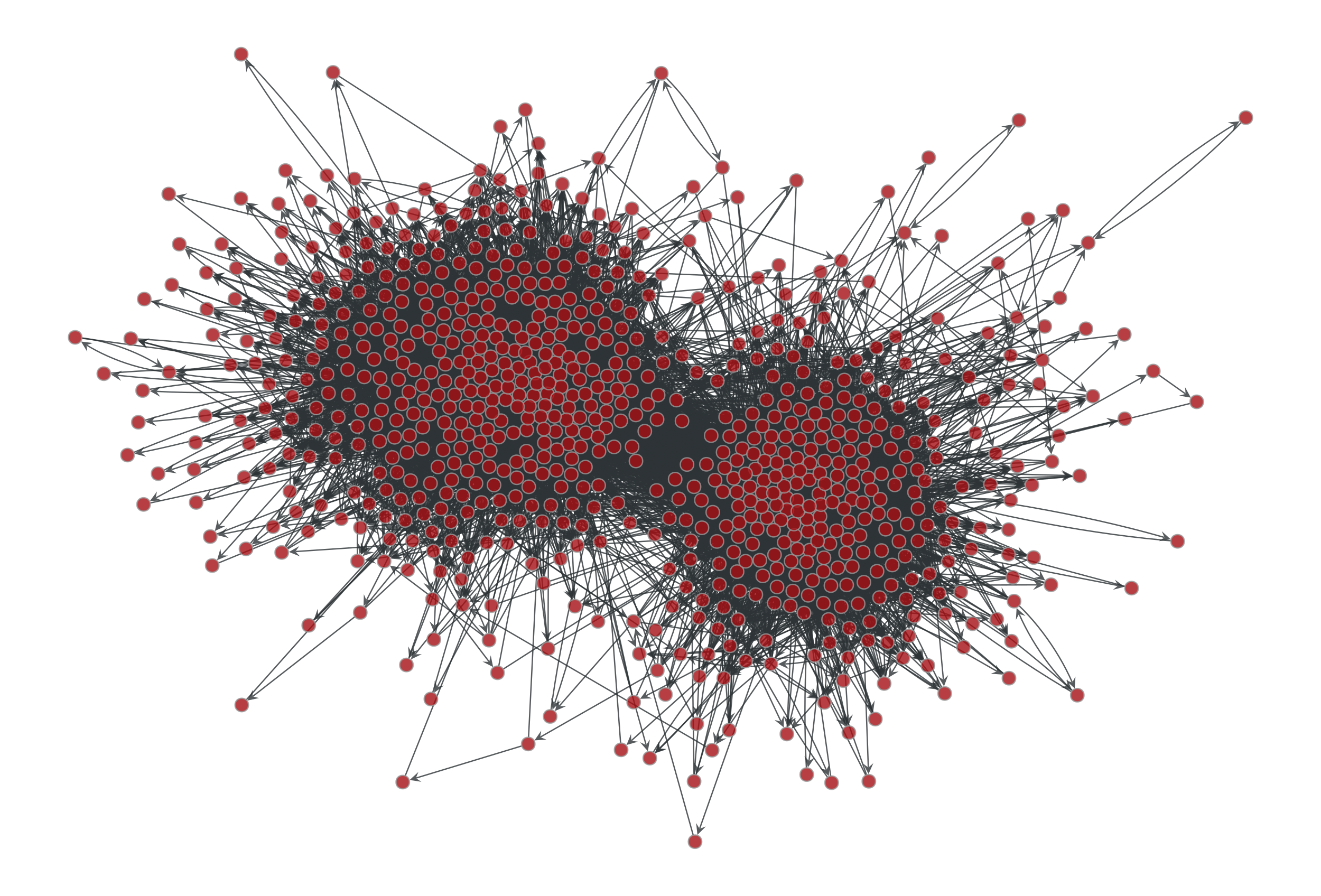
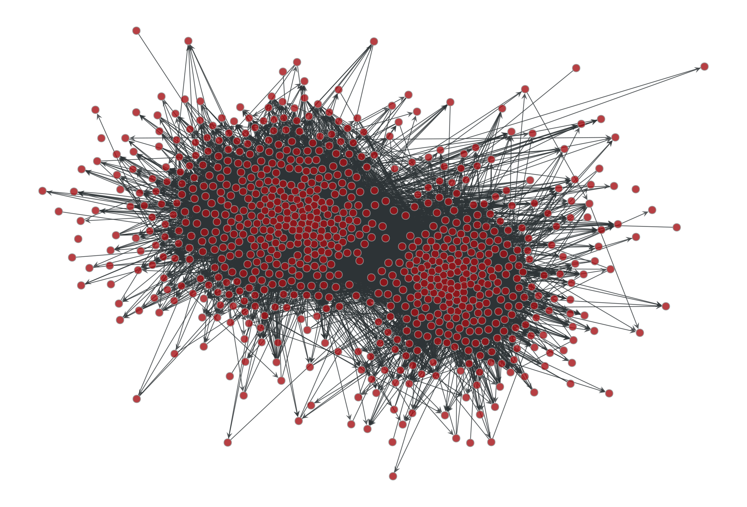
Left: Political blogs network. Right: Sample from the maximum-entropy degree-corrected SBM fitted to the original network.