random_graph

graph_tool.generation.random_graph(N, deg_sampler, directed=True, parallel_edges=False, self_loops=False, block_membership=None, block_type='int', degree_block=False, random=True, verbose=False, **kwargs)

Generate a random graph, with a given degree distribution and (optionally) vertex-vertex correlation.

The graph will be randomized via the random_rewire() function, and any remaining parameters will be passed to that function. Please read its documentation for all the options regarding the different statistical models which can be chosen.

Parameters:

Nint

Number of vertices in the graph.

deg_samplerfunction

A degree sampler function which is called without arguments, and returns a tuple of ints representing the in and out-degree of a given vertex (or a single int for undirected graphs, representing the out-degree). This function is called once per vertex, but may be called more times, if the degree sequence cannot be used to build a graph.

Optionally, you can also pass a function which receives one or two arguments. If block_membership is None, the single argument passed will be the index of the vertex which will receive the degree. If block_membership is not None, the first value passed will be the vertex index, and the second will be the block value of the vertex.

directedbool (optional, default: True)

Whether the generated graph should be directed.

parallel_edgesbool (optional, default: False)

If True, parallel edges are allowed.

self_loopsbool (optional, default: False)

If True, self-loops are allowed.

block_membershiplist or numpy.ndarray or function (optional, default: None)

If supplied, the graph will be sampled from a stochastic blockmodel ensemble, and this parameter specifies the block membership of the vertices, which will be passed to the random_rewire() function.

If the value is a list or a numpy.ndarray, it must have len(block_membership) == N, and the values will define to which block each vertex belongs.

If this value is a function, it will be used to sample the block types. It must be callable either with no arguments or with a single argument which will be the vertex index. In either case it must return a type compatible with the block_type parameter.

See the documentation for the vertex_corr parameter of the random_rewire() function which specifies the correlation matrix.

block_typestring (optional, default: "int")

Value type of block labels. Valid only if block_membership is not None.

degree_blockbool (optional, default: False)

If True, the degree of each vertex will be appended to block labels when constructing the blockmodel, such that the resulting block type will be a pair \((r, k)\), where \(r\) is the original block label.

randombool (optional, default: True)

If True, the returned graph is randomized. Otherwise a deterministic placement of the edges will be used.

verbosebool (optional, default: False)

If True, verbose information is displayed.

Returns:

random_graphGraph

The generated graph.

blocksVertexPropertyMap

A vertex property map with the block values. This is only returned if block_membership is not None.

See also

random_rewire

in-place graph shuffling

Notes

The algorithm makes sure the degree sequence is graphical (i.e. realizable) and keeps re-sampling the degrees if is not. With a valid degree sequence, the edges are placed deterministically, and later the graph is shuffled with the random_rewire() function, with all remaining parameters passed to it.

The complexity is \(O(V + E)\) if parallel edges are allowed, and \(O(V + E \times\text{n-iter})\) if parallel edges are not allowed.

Note

If parallel_edges == False this algorithm only guarantees that the returned graph will be a random sample from the desired ensemble if n_iter is sufficiently large. The algorithm implements an efficient Markov chain based on edge swaps, with a mixing time which depends on the degree distribution and correlations desired. If degree correlations are provided, the mixing time tends to be larger.

References

[metropolis-equations-1953]

Metropolis, N.; Rosenbluth, A.W.; Rosenbluth, M.N.; Teller, A.H.; Teller, E. “Equations of State Calculations by Fast Computing Machines”. Journal of Chemical Physics 21 (6): 1087-1092 (1953). DOI: 10.1063/1.1699114 [sci-hub, @tor]

[hastings-monte-carlo-1970]

Hastings, W.K. “Monte Carlo Sampling Methods Using Markov Chains and Their Applications”. Biometrika 57 (1): 97-109 (1970). DOI: 10.1093/biomet/57.1.97 [sci-hub, @tor]

[holland-stochastic-1983]

Paul W. Holland, Kathryn Blackmond Laskey, and Samuel Leinhardt, “Stochastic blockmodels: First steps,” Social Networks 5, no. 2: 109-13 (1983) DOI: 10.1016/0378-8733(83)90021-7 [sci-hub, @tor]

[karrer-stochastic-2011]

Brian Karrer and M. E. J. Newman, “Stochastic blockmodels and community structure in networks,” Physical Review E 83, no. 1: 016107 (2011) DOI: 10.1103/PhysRevE.83.016107 [sci-hub, @tor] arXiv: 1008.3926

Examples

This is a degree sampler which uses rejection sampling to sample from the distribution \(P(k)\propto 1/k\), up to a maximum.

>>> def sample_k(max):
...     accept = False
...     while not accept:
...         k = np.random.randint(1,max+1)
...         accept = np.random.random() < 1.0/k
...     return k

The following generates a random undirected graph with degree distribution \(P(k)\propto 1/k\) (with k_max=40) and an assortative degree correlation of the form:

\[P(i,k) \propto \frac{1}{1+|i-k|}\]

>>> g = gt.random_graph(1000, lambda: sample_k(40), model="probabilistic-configuration",
...                     edge_probs=lambda i, k: 1.0 / (1 + abs(i - k)), directed=False,
...                     n_iter=100)

The following samples an in,out-degree pair from the joint distribution:

\[p(j,k) = \frac{1}{2}\frac{e^{-m_1}m_1^j}{j!}\frac{e^{-m_1}m_1^k}{k!} + \frac{1}{2}\frac{e^{-m_2}m_2^j}{j!}\frac{e^{-m_2}m_2^k}{k!}\]

with \(m_1 = 4\) and \(m_2 = 20\).

>>> def deg_sample():
...    if random() > 0.5:
...        return np.random.poisson(4), np.random.poisson(4)
...    else:
...        return np.random.poisson(20), np.random.poisson(20)
...

The following generates a random directed graph with this distribution, and plots the combined degree correlation.

>>> g = gt.random_graph(20000, deg_sample)
>>>
>>> hist = gt.combined_corr_hist(g, "in", "out")
>>>
>>> figure()
<...>
>>> imshow(hist[0].T, interpolation="nearest", origin="lower")
<...>
>>> colorbar()
<...>
>>> xlabel("in-degree")
Text(...)
>>> ylabel("out-degree")
Text(...)
>>> tight_layout()
>>> savefig("combined-deg-hist.svg")

Combined degree histogram.

A correlated directed graph can be build as follows. Consider the following degree correlation:

\[P(j',k'|j,k)=\frac{e^{-k}k^{j'}}{j'!} \frac{e^{-(20-j)}(20-j)^{k'}}{k'!}\]

i.e., the in->out correlation is “disassortative”, the out->in correlation is “assortative”, and everything else is uncorrelated. We will use a flat degree distribution in the range [1,20).

>>> p = scipy.stats.poisson
>>> g = gt.random_graph(20000, lambda: (sample_k(19), sample_k(19)),
...                     model="probabilistic-configuration",
...                     edge_probs=lambda a,b: (p.pmf(a[0], b[1]) *
...                                             p.pmf(a[1], 20 - b[0])),
...                     n_iter=100)

Lets plot the average degree correlations to check.

>>> figure(figsize=(8,3))
<...>
>>> corr = gt.avg_neighbor_corr(g, "in", "in")
>>> errorbar(corr[2][:-1], corr[0], yerr=corr[1], fmt="o-",
...         label=r"$\left<\text{in}\right>$ vs in")
<...>
>>> corr = gt.avg_neighbor_corr(g, "in", "out")
>>> errorbar(corr[2][:-1], corr[0], yerr=corr[1], fmt="o-",
...         label=r"$\left<\text{out}\right>$ vs in")
<...>
>>> corr = gt.avg_neighbor_corr(g, "out", "in")
>>> errorbar(corr[2][:-1], corr[0], yerr=corr[1], fmt="o-",
...          label=r"$\left<\text{in}\right>$ vs out")
<...>
>>> corr = gt.avg_neighbor_corr(g, "out", "out")
>>> errorbar(corr[2][:-1], corr[0], yerr=corr[1], fmt="o-",
...          label=r"$\left<\text{out}\right>$ vs out")
<...>
>>> legend(loc='center left', bbox_to_anchor=(1, 0.5))
<...>
>>> xlabel("Source degree")
Text(...)
>>> ylabel("Average target degree")
Text(...)
>>> tight_layout()
>>> box = gca().get_position()
>>> gca().set_position([box.x0, box.y0, box.width * 0.7, box.height])
>>> savefig("deg-corr-dir.svg")

Average nearest neighbor correlations.

Stochastic blockmodels

The following example shows how a stochastic blockmodel [holland-stochastic-1983] [karrer-stochastic-2011] can be generated. We will consider a system of 10 blocks, which form communities. The connection probability will be given by

>>> def prob(a, b):
...    if a == b:
...        return 0.999
...    else:
...        return 0.001

The blockmodel can be generated as follows.

>>> g, bm = gt.random_graph(2000, lambda: poisson(10), directed=False,
...                         model="blockmodel",
...                         block_membership=lambda: randint(10),
...                         edge_probs=prob)
>>> gt.graph_draw(g, vertex_fill_color=bm, edge_color="black", output="blockmodel.pdf")
<...>

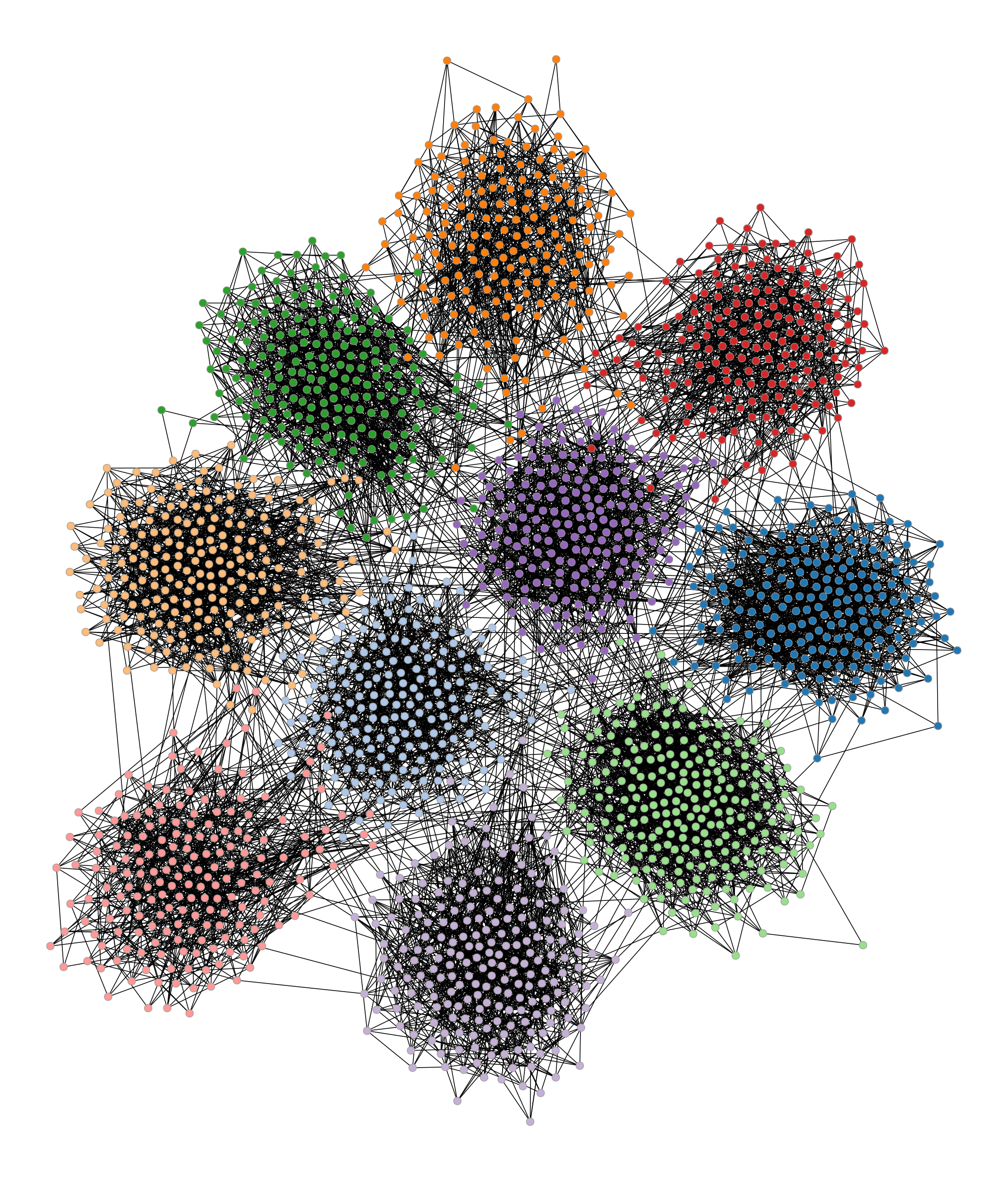
Simple blockmodel with 10 blocks.