betweenness#
- graph_tool.centrality.betweenness(g, pivots=None, vprop=None, eprop=None, weight=None, norm=True)[source]#
Calculate the betweenness centrality for each vertex and edge.
- Parameters:
- g
Graph Graph to be used.
- pivotslist or
numpy.ndarray, optional (default: None) If provided, the betweenness will be estimated using the vertices in this list as pivots. If the list contains all nodes (the default) the algorithm will be exact, and if the vertices are randomly chosen the result will be an unbiased estimator.
- vprop
VertexPropertyMap, optional (default: None) Vertex property map to store the vertex betweenness values.
- eprop
EdgePropertyMap, optional (default: None) Edge property map to store the edge betweenness values.
- weight
EdgePropertyMap, optional (default: None) Edge property map corresponding to the weight value of each edge.
- normbool, optional (default: True)
Whether or not the betweenness values should be normalized.
- g
- Returns:
- vertex_betweennessA vertex property map with the vertex betweenness values.
- edge_betweennessAn edge property map with the edge betweenness values.
See also
central_point_dominancecentral point dominance of the graph
pagerankPageRank centrality
eigentrusteigentrust centrality
eigenvectoreigenvector centrality
hitsauthority and hub centralities
trust_transitivitypervasive trust transitivity
Notes
Betweenness centrality of a vertex \(C_B(v)\) is defined as,
\[C_B(v)= \sum_{s \neq v \neq t \in V \atop s \neq t} \frac{\sigma_{st}(v)}{\sigma_{st}}\]where \(\sigma_{st}\) is the number of shortest paths from s to t, and \(\sigma_{st}(v)\) is the number of shortest paths from s to t that pass through a vertex \(v\). This may be normalised by dividing through the number of pairs of vertices not including v, which is \((n-1)(n-2)/2\), for undirected graphs, or \((n-1)(n-2)\) for directed ones.
The algorithm used here is defined in [brandes-faster-2001], and has a complexity of \(O(VE)\) for unweighted graphs and \(O(VE + V(V+E)\log V)\) for weighted graphs. The space complexity is \(O(VE)\).
If the
pivotsparameter is given, the complexity will be instead \(O(PE)\) for unweighted graphs and \(O(PE + P(V+E)\log V)\) for weighted graphs, where \(P\) is the number of pivot vertices.Parallel implementation.
If enabled during compilation, this algorithm will run in parallel using OpenMP. See the parallel algorithms section for information about how to control several aspects of parallelization.
References
[betweenness-wikipedia]http://en.wikipedia.org/wiki/Centrality#Betweenness_centrality
[brandes-faster-2001]U. Brandes, “A faster algorithm for betweenness centrality”, Journal of Mathematical Sociology, 2001, DOI: 10.1080/0022250X.2001.9990249 [sci-hub, @tor]
[brandes-centrality-2007]U. Brandes, C. Pich, “Centrality estimation in large networks”, Int. J. Bifurcation Chaos 17, 2303 (2007). DOI: 10.1142/S0218127407018403 [sci-hub, @tor]
[adamic-polblogs]L. A. Adamic and N. Glance, “The political blogosphere and the 2004 US Election”, in Proceedings of the WWW-2005 Workshop on the Weblogging Ecosystem (2005). DOI: 10.1145/1134271.1134277 [sci-hub, @tor]
Examples
>>> g = gt.collection.data["polblogs"]
>>> g = gt.GraphView(g, vfilt=gt.label_largest_component(g))
>>> vp, ep = gt.betweenness(g)
>>> gt.graph_draw(g, pos=g.vp["pos"], vertex_fill_color=vp,
...               vertex_size=gt.prop_to_size(vp, mi=5, ma=15),
...               edge_pen_width=gt.prop_to_size(ep, mi=0.5, ma=5),
...               vcmap=matplotlib.cm.gist_heat,
...               vorder=vp, output="polblogs_betweenness.pdf")
<...>
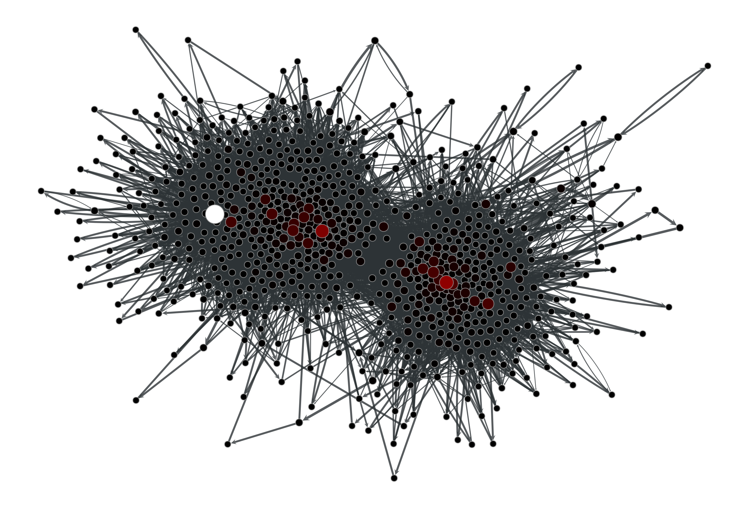
Betweenness values of the a political blogs network of [adamic-polblogs].#