price_network

graph_tool.generation.price_network(N, m=1, c=None, gamma=1, directed=True, seed_graph=None)

A generalized version of Price’s — or Barabási-Albert if undirected — preferential attachment network model.

Parameters:

Nint

Size of the network.

mint (optional, default: 1)

Out-degree of newly added vertices.

cfloat (optional, default: 1 if directed == True else 0)

Constant factor added to the probability of a vertex receiving an edge (see notes below).

gammafloat (optional, default: 1)

Preferential attachment exponent (see notes below).

directedbool (optional, default: True)

If True, a Price network is generated. If False, a Barabási-Albert network is generated.

seed_graphGraph (optional, default: None)

If provided, this graph will be used as the starting point of the algorithm.

Returns:

price_graphGraph

The generated graph.

See also

triangulation

2D or 3D triangulation

random_graph

random graph generation

lattice

N-dimensional square lattice

geometric_graph

N-dimensional geometric network

Notes

The (generalized) [price] network is either a directed or undirected graph (the latter is called a Barabási-Albert network), generated dynamically by at each step adding a new vertex, and connecting it to \(m\) other vertices, chosen with probability \(\pi\) defined as:

\[\pi \propto k^\gamma + c\]

where \(k\) is the (in-)degree of the vertex (or simply the degree in the undirected case).

Note that for directed graphs we must have \(c \ge 0\), and for undirected graphs, \(c > -\min(k_{\text{min}}, m)^{\gamma}\), where \(k_{\text{min}}\) is the smallest degree in the seed graph.

If \(\gamma=1\), the tail of resulting in-degree distribution of the directed case is given by

\[P_{k_\text{in}} \sim k_\text{in}^{-(2 + c/m)},\]

or for the undirected case

\[P_{k} \sim k^{-(3 + c/m)}.\]

However, if \(\gamma \ne 1\), the in-degree distribution is not scale-free (see [dorogovtsev-evolution] for details).

Note that if seed_graph is not given, the algorithm will always start with one vertex if \(c > 0\), or with two vertices with an edge between them otherwise. If \(m > 1\), the degree of the newly added vertices will be vary dynamically as \(m'(t) = \min(m, V(t))\), where \(V(t)\) is the number of vertices added so far. If this behaviour is undesired, a proper seed graph with \(V \ge m\) vertices must be provided.

This algorithm runs in \(O(V\log V)\) time.

References

[yule]

Yule, G. U. “A Mathematical Theory of Evolution, based on the Conclusions of Dr. J. C. Willis, F.R.S.”. Philosophical Transactions of the Royal Society of London, Ser. B 213: 21-87, 1925, DOI: 10.1098/rstb.1925.0002 [sci-hub, @tor]

[price]

Derek De Solla Price, “A general theory of bibliometric and other cumulative advantage processes”, Journal of the American Society for Information Science, Volume 27, Issue 5, pages 292-306, September 1976, DOI: 10.1002/asi.4630270505 [sci-hub, @tor]

[barabasi-albert]

Barabási, A.-L., and Albert, R., “Emergence of scaling in random networks”, Science, 286, 509, 1999, DOI: 10.1126/science.286.5439.509 [sci-hub, @tor]

[dorogovtsev-evolution]

S. N. Dorogovtsev and J. F. F. Mendes, “Evolution of networks”, Advances in Physics, 2002, Vol. 51, No. 4, 1079-1187, DOI: 10.1080/00018730110112519 [sci-hub, @tor]

Examples

>>> g = gt.price_network(20000)
>>> gt.graph_draw(g, pos=gt.sfdp_layout(g, cooling_step=0.99),
...               vertex_fill_color=g.vertex_index, vertex_size=2,
...               vcmap=matplotlib.cm.plasma,
...               edge_pen_width=1, output="price-network.pdf")
<...>
>>> g = gt.price_network(20000, c=0.1)
>>> gt.graph_draw(g, pos=gt.sfdp_layout(g, cooling_step=0.99),
...               vertex_fill_color=g.vertex_index, vertex_size=2,
...               vcmap=matplotlib.cm.plasma,
...               edge_pen_width=1, output="price-network-broader.pdf")
<...>

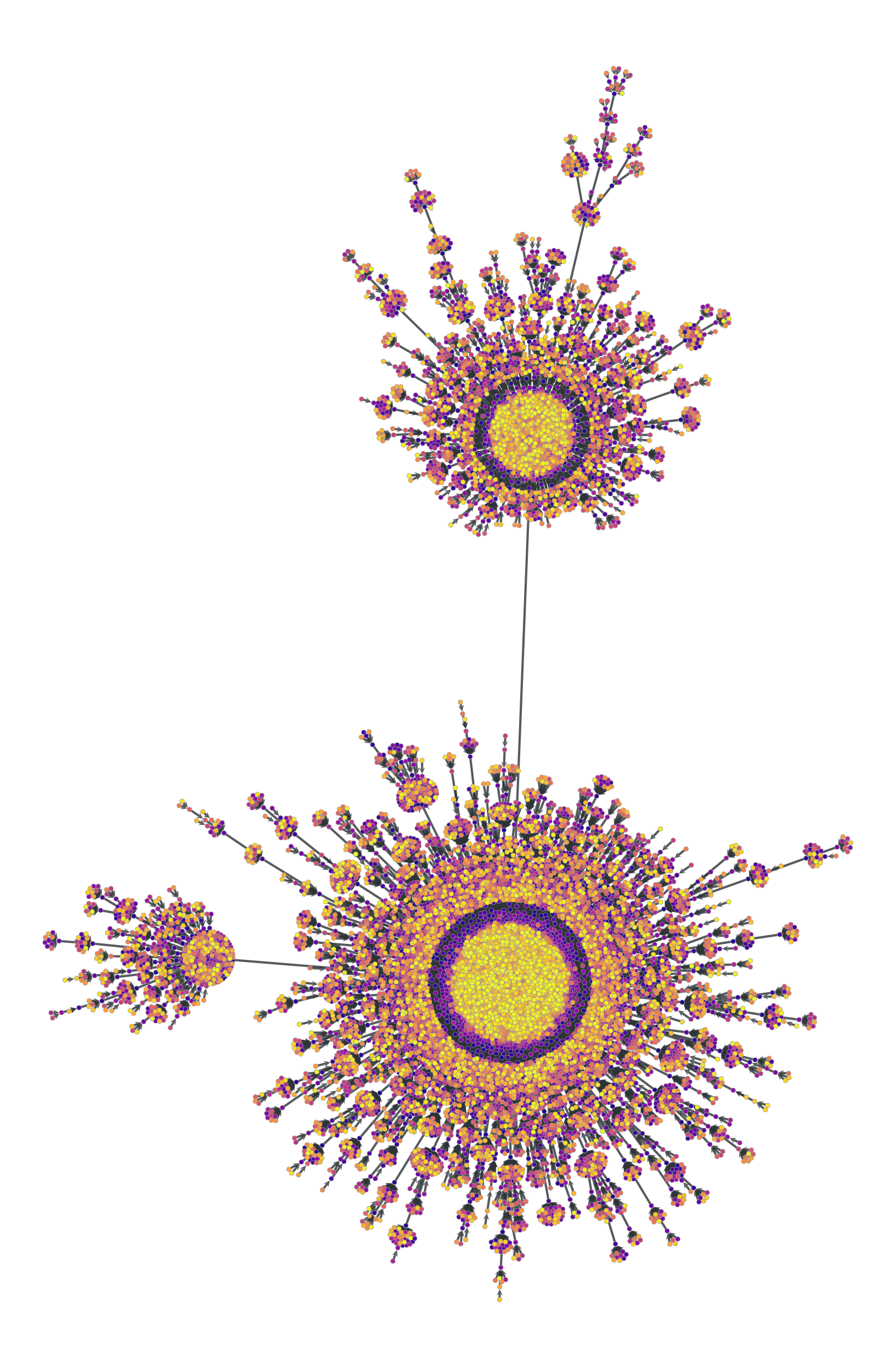
Price network with \(N=2\times 10^4\) nodes and \(c=1\). The colors represent the order in which vertices were added.

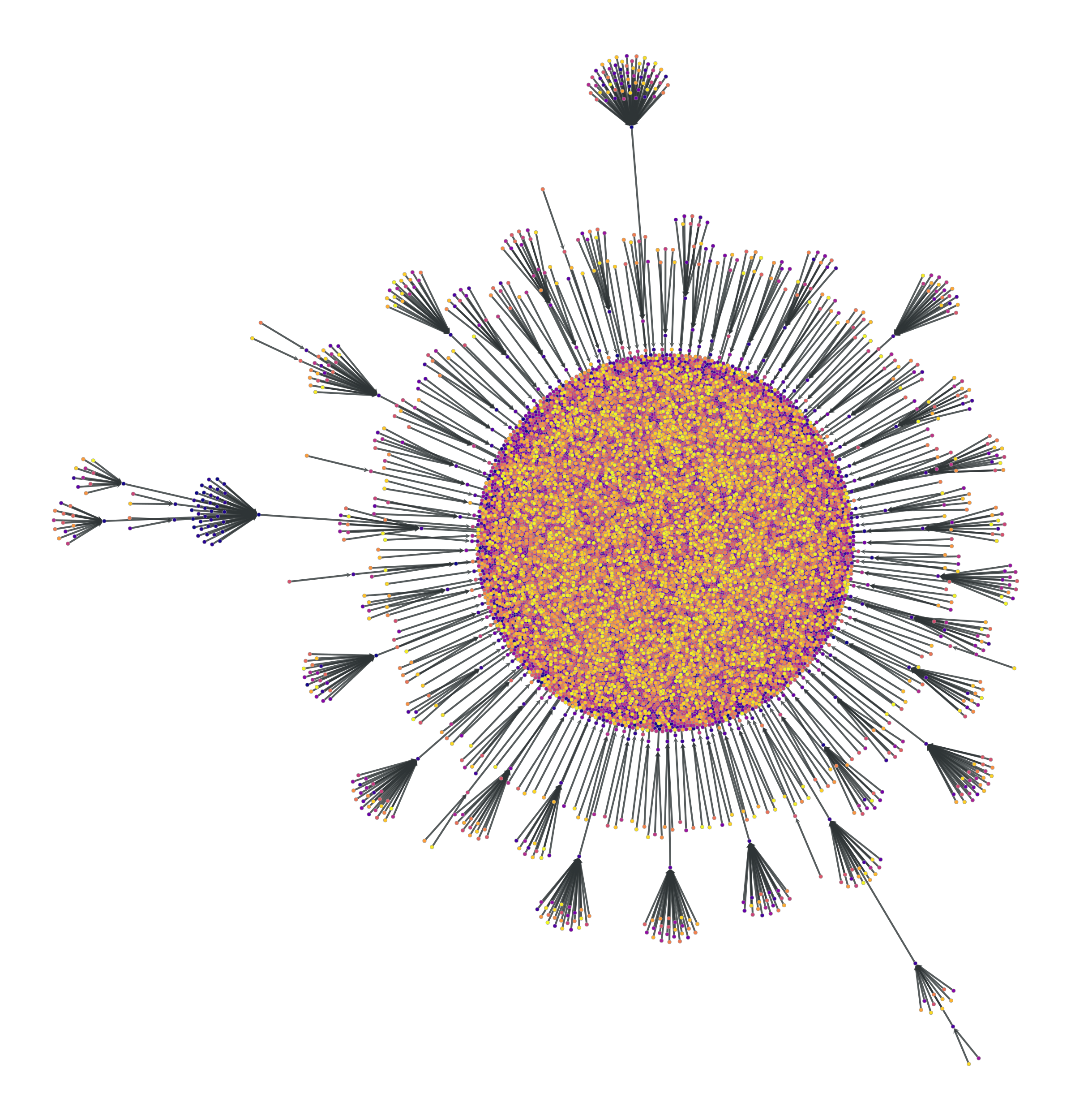
Price network with \(N=2\times 10^4\) nodes and \(c=0.1\). The colors represent the order in which vertices were added.