generate_sbm

graph_tool.generation.generate_sbm(b, probs, out_degs=None, in_degs=None, directed=False, micro_ers=False, micro_degs=False)

Generate a random graph by sampling from the Poisson or microcanonical stochastic block model.

Parameters:

biterable or numpy.ndarray

Group membership for each vertex.

probstwo-dimensional numpy.ndarray or scipy.sparse.spmatrix

Matrix with edge propensities between groups. The value probs[r,s] corresponds to the average number of edges between groups r and s (or twice the average number if r == s and the graph is undirected).

out_degsiterable or numpy.ndarray (optional, default: None)

Out-degree propensity for each vertex. If not provided, a constant value will be used. Note that the values will be normalized inside each group, if they are not already so.

in_degsiterable or numpy.ndarray (optional, default: None)

In-degree propensity for each vertex. If not provided, a constant value will be used. Note that the values will be normalized inside each group, if they are not already so.

directedbool (optional, default: False)

Whether the graph is directed.

micro_ersbool (optional, default: False)

If true, the microcanonical version of the model will be evoked, where the numbers of edges between groups will be given exactly by the parameter probs, and this will not fluctuate between samples.

micro_degsbool (optional, default: False)

If true, the microcanonical version of the degree-corrected model will be evoked, where the degrees of vertices will be given exactly by the parameters out_degs and in_degs, and they will not fluctuate between samples. (If micro_degs == True it implies micro_ers == True.)

Returns:

gGraph

The generated graph.

See also

random_graph

random graph generation

Notes

The algorithm generates multigraphs with self-loops, according to the Poisson degree-corrected stochastic block model (SBM) [karrer-stochastic-2011], which includes the traditional SBM as a special case.

The multigraphs are generated with probability

\[P({\boldsymbol A}|{\boldsymbol \theta},{\boldsymbol \lambda},{\boldsymbol b}) = \prod_{i<j}\frac{e^{-\lambda_{b_ib_j}\theta_i\theta_j}(\lambda_{b_ib_j}\theta_i\theta_j)^{A_{ij}}}{A_{ij}!} \times\prod_i\frac{e^{-\lambda_{b_ib_i}\theta_i^2/2}(\lambda_{b_ib_i}\theta_i^2/2)^{A_{ij}/2}}{(A_{ij}/2)!},\]

where \(\lambda_{rs}\) is the edge propensity between groups \(r\) and \(s\), and \(\theta_i\) is the propensity of vertex i to receive edges, which is proportional to its expected degree. Note that in the algorithm it is assumed that the vertex propensities are normalized for each group,

\[\sum_i\theta_i\delta_{b_i,r} = 1,\]

such that the value \(\lambda_{rs}\) will correspond to the average number of edges between groups \(r\) and \(s\) (or twice that if \(r = s\)). If the supplied values of \(\theta_i\) are not normalized as above, they will be normalized prior to the generation of the graph.

For directed graphs, the probability is analogous, with \(\lambda_{rs}\) being in general asymmetric:

\[P({\boldsymbol A}|{\boldsymbol \theta},{\boldsymbol \lambda},{\boldsymbol b}) = \prod_{ij}\frac{e^{-\lambda_{b_ib_j}\theta^+_i\theta^-_j}(\lambda_{b_ib_j}\theta^+_i\theta^-_j)^{A_{ij}}}{A_{ij}!}.\]

Again, the same normalization is assumed:

\[\sum_i\theta_i^+\delta_{b_i,r} = \sum_i\theta_i^-\delta_{b_i,r} = 1,\]

such that the value \(\lambda_{rs}\) will correspond to the average number of directed edges between groups \(r\) and \(s\).

The traditional (i.e. non-degree-corrected) SBM is recovered from the above model by setting \(\theta_i=1/n_{b_i}\) (or \(\theta^+_i=\theta^-_i=1/n_{b_i}\) in the directed case), which is done automatically if out_degs and in_degs are not specified.

In case the parameter micro_degs == True is passed, a microcanical model is used instead, where both the number of edges between groups as well as the degrees of the vertices are preserved exactly, instead of only on expectation [peixoto-nonparametric-2017]. In this case, the parameters are interpreted as \({\boldsymbol\lambda}\equiv{\boldsymbol e}\) and \({\boldsymbol\theta}\equiv{\boldsymbol k}\), where \(e_{rs}\) is the number of edges between groups \(r\) and \(s\) (or twice that if \(r=s\) in the undirected case), and \(k_i\) is the degree of vertex \(i\). This model is a generalization of the configuration model, where multigraphs are sampled with probability

\[P({\boldsymbol A}|{\boldsymbol k},{\boldsymbol e},{\boldsymbol b}) = \frac{\prod_{r<s}e_{rs}!\prod_re_{rr}!!\prod_ik_i!}{\prod_re_r!\prod_{i<j}A_{ij}!\prod_iA_{ii}!!}.\]

and in the directed case with probability

\[P({\boldsymbol A}|{\boldsymbol k}^+,{\boldsymbol k}^-,{\boldsymbol e},{\boldsymbol b}) = \frac{\prod_{rs}e_{rs}!\prod_ik^+_i!k^-_i!}{\prod_re^+_r!e^-_r!\prod_{ij}A_{ij}!}.\]

where \(e^+_r = \sum_se_{rs}\), \(e^-_r = \sum_se_{sr}\), \(k^+_i = \sum_jA_{ij}\) and \(k^-_i = \sum_jA_{ji}\).

In the non-degree-corrected case, if micro_ers == True, the microcanonical model corresponds to

\[P({\boldsymbol A}|{\boldsymbol e},{\boldsymbol b}) = \frac{\prod_{r<s}e_{rs}!\prod_re_{rr}!!}{\prod_rn_r^{e_r}\prod_{i<j}A_{ij}!\prod_iA_{ii}!!},\]

and in the directed case to

\[P({\boldsymbol A}|{\boldsymbol e},{\boldsymbol b}) = \frac{\prod_{rs}e_{rs}!}{\prod_rn_r^{e_r^+ + e_r^-}\prod_{ij}A_{ij}!}.\]

In every case above, the final graph is generated in time \(O(V + E + B)\), where \(B\) is the number of groups.

References

[karrer-stochastic-2011]

Brian Karrer and M. E. J. Newman, “Stochastic blockmodels and community structure in networks,” Physical Review E 83, no. 1: 016107 (2011) DOI: 10.1103/PhysRevE.83.016107 [sci-hub, @tor] arXiv: 1008.3926

[peixoto-nonparametric-2017]

Tiago P. Peixoto, “Nonparametric Bayesian inference of the microcanonical stochastic block model”, Phys. Rev. E 95 012317 (2017). DOI: 10.1103/PhysRevE.95.012317 [sci-hub, @tor], arXiv: 1610.02703

Examples

>>> g = gt.collection.data["polblogs"]
>>> g = gt.GraphView(g, vfilt=gt.label_largest_component(g))
>>> g = gt.Graph(g, prune=True)
>>> state = gt.minimize_blockmodel_dl(g)
>>> u = gt.generate_sbm(state.b.a, gt.adjacency(state.get_bg(),
...                                             state.get_ers()).T,
...                     g.degree_property_map("out").a,
...                     g.degree_property_map("in").a, directed=True)
>>> gt.graph_draw(g, g.vp.pos, output="polblogs-sbm.pdf")
<...>
>>> gt.graph_draw(u, u.own_property(g.vp.pos), output="polblogs-sbm-generated.pdf")
<...>

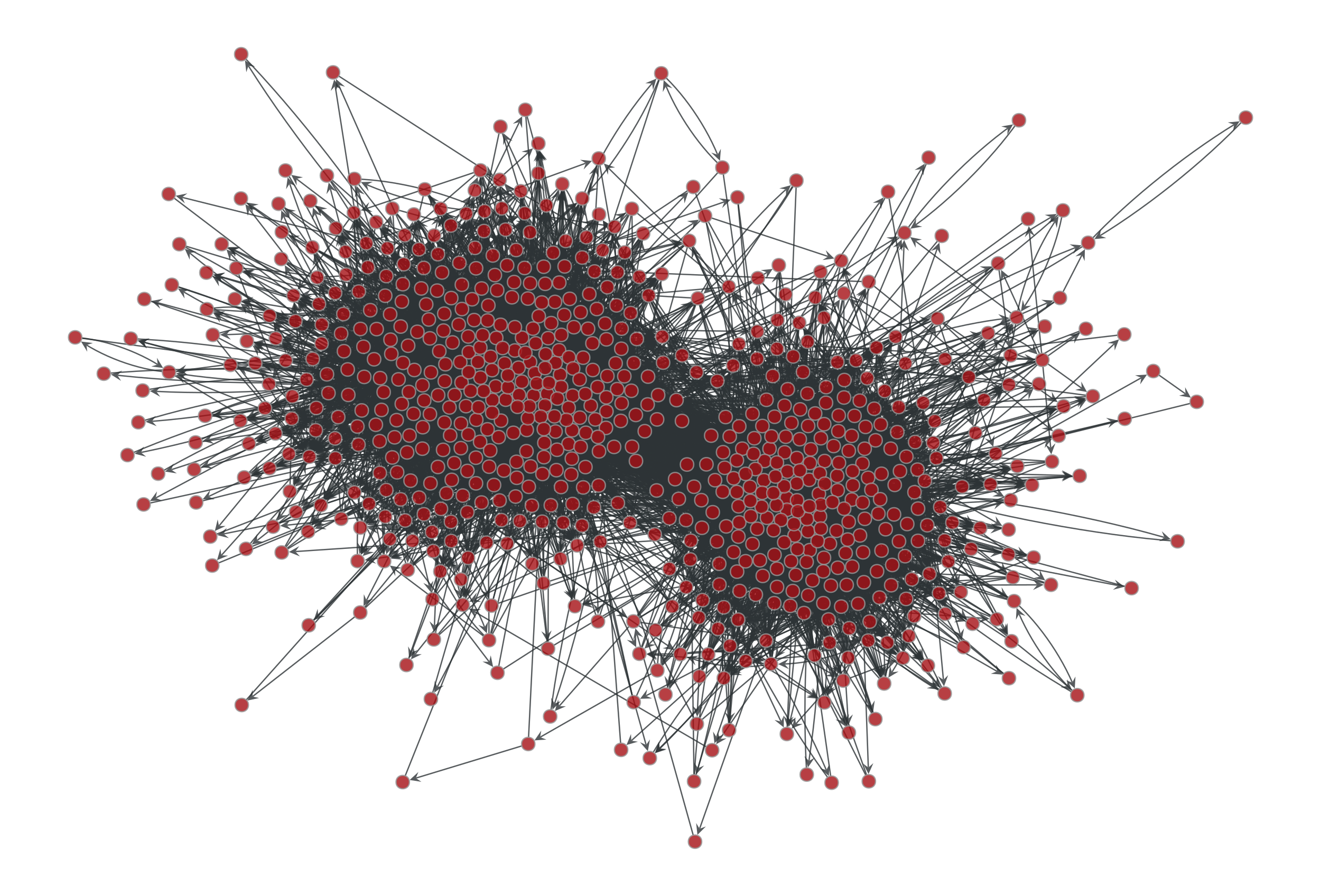
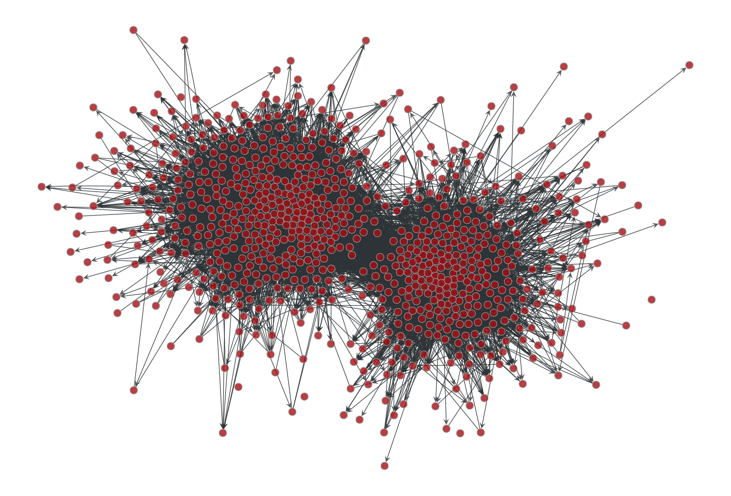
Left: Political blogs network. Right: Sample from the degree-corrected SBM fitted to the original network.